imdb nn-model Published by onesixx 19-05-09 19-05-09
##3# Build the model -----------------------------------------------------------
trn_Data %>% dim() # [1] 25000 10000
## ` ` Setup the layers --------------------------------------------------------
model <- keras_model_sequential() %>%
layer_dense(units=16, activation="relu", input_shape=c(10000)) %>%
layer_dense(units=16, activation="relu") %>%
layer_dense(units= 1, activation="sigmoid")
model %>% summary()
# _________________________________________________________
# Layer (type) Output Shape Param #
# =========================================================
# dense_1 (Dense) (None, 16) 160016 10000*16 + 16
# _________________________________________________________
# dense_2 (Dense) (None, 16) 272 16*16 + 16
# _________________________________________________________
# dense_3 (Dense) (None, 1) 17 16*1 + 1
# =========================================================
# Total params: 160,305
# Trainable params: 160,305
# Non-trainable params: 0
# _________________________________________________________
## ` ` Compile the model -------------------------------------------------------
model %>% compile(
optimizer="rmsprop", #optimizer_rmsprop(lr=.001)
loss="binary_crossentropy",
metrics=c("accuracy")
)
##4# Train the model -----------------------------------------------------------
# Validating your approach ~~~~~~~~
# validation set
val_indices <- 1:10000 # 40%
trn_Data_validate <- trn_Data[ val_indices, ]
trn_Data_partial <- trn_Data[-val_indices, ]
trn_Labels_validate<- trn_Labels[ val_indices]
trn_Labels_partial <- trn_Labels[-val_indices]
history <- model %>% fit( # fit.keras.engine.training.Model
x=trn_Data_partial,
y=trn_Labels_partial,
batch_size=512,
epoches=20,
validation_data= list(trn_Data_validate, trn_Labels_validate)
)
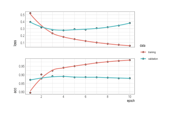
history %>% plot()
p <- as.data.table(history) %>% ggplot(aes(x=epoch, y=value, group=data, color=data)) +
                              geom_point(size=.6) + geom_line()  +
                              stat_peaks(colour="red")+
                              stat_peaks(geom="text", colour="red", vjust=-0.5, check_overlap=T, span=NULL)+
                              stat_valleys(colour="blue")+
                              stat_valleys(geom="text", colour="blue", vjust=-0.5, check_overlap=T, span=NULL)+
                              facet_grid(metric~.)
p
ggplotly(p)

p1 <- as.data.table(history) %>% ggplot(aes(x=epoch, y=value, group=metric, color=metric)) +
                                  geom_point() + geom_line() + facet_grid(data~.)
p1
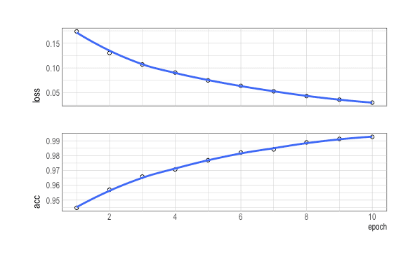
# train2 from beginning
history <- model %>% fit(  # fit.keras.engine.training.Model
  x=trn_Data,
  y=trn_Labels,
  batch_size=512,
  epoches=4,
  #validation_data= list(trn_Data_validate, trn_Labels_validate)
)
history %>% plot()
##5# Evaluate accuracy ---------------------------------------------------------
# retraining with proper epoches
model %>% fit(
  x=trn_Data_partial,
  y=trn_Labels_partial,
  batch_size=512,
  epoches=4         # prevent overfitting
)

results <- model %>% evaluate(tst_Data, tst_Labels)
results

##6# Make predictions ----------------------------------------------------------
model %>% predict(tst_Data[1:10, ])

pred <- model %>% predict(tst_Data)
pred %>% plot()
sum(pred>0.9 | pred<0.1) / length(pred)    # 0.85768
#~~~~~~~~~~~~~~~~~~~~~~~~~~~~~~~~~~~~~~~~~~~~~~~~~~~~~~~~~~~~~~~~~~~~~~~~~~~~~~~
#  Further experiments
# hidden layers 2 --> try 3
model <- keras_model_sequential() %>%
  layer_dense(units=64, activation="relu", input_shape=c(10000)) %>%
  layer_dense(units=16, activation="relu") %>%
  layer_dense(units=16, activation="relu") %>%
  layer_dense(units= 1, activation="sigmoid")

model <- keras_model_sequential() %>%
  layer_dense(units=32, activation="tanh", input_shape=c(10000)) %>%
  layer_dense(units=16, activation="tanh") %>%
  layer_dense(units=16, activation="tanh") %>%
  layer_dense(units= 1, activation="sigmoid")

model %>% compile(
  optimizer="rmsprop",
  loss="mse", #"binary_crossentropy",
  metrics=c("accuracy")
)

history <- model %>% fit(
  x=trn_Data,
  y=trn_Labels,
  batch_size=512,
  epoches=6,
  #validation_data= list(trn_Data_validate, trn_Labels_validate)
)
history %>% plot()

##6# Make predictions ----------------------------------------------------------
model %>% evaluate(tst_Data, tst_Labels)
pred <- model %>% predict(tst_Data)