DNN (Deep Neural Network)

Published onesixx on 19-05-0119-05-01

neuralnet, nnet, deepnet

Neural Network

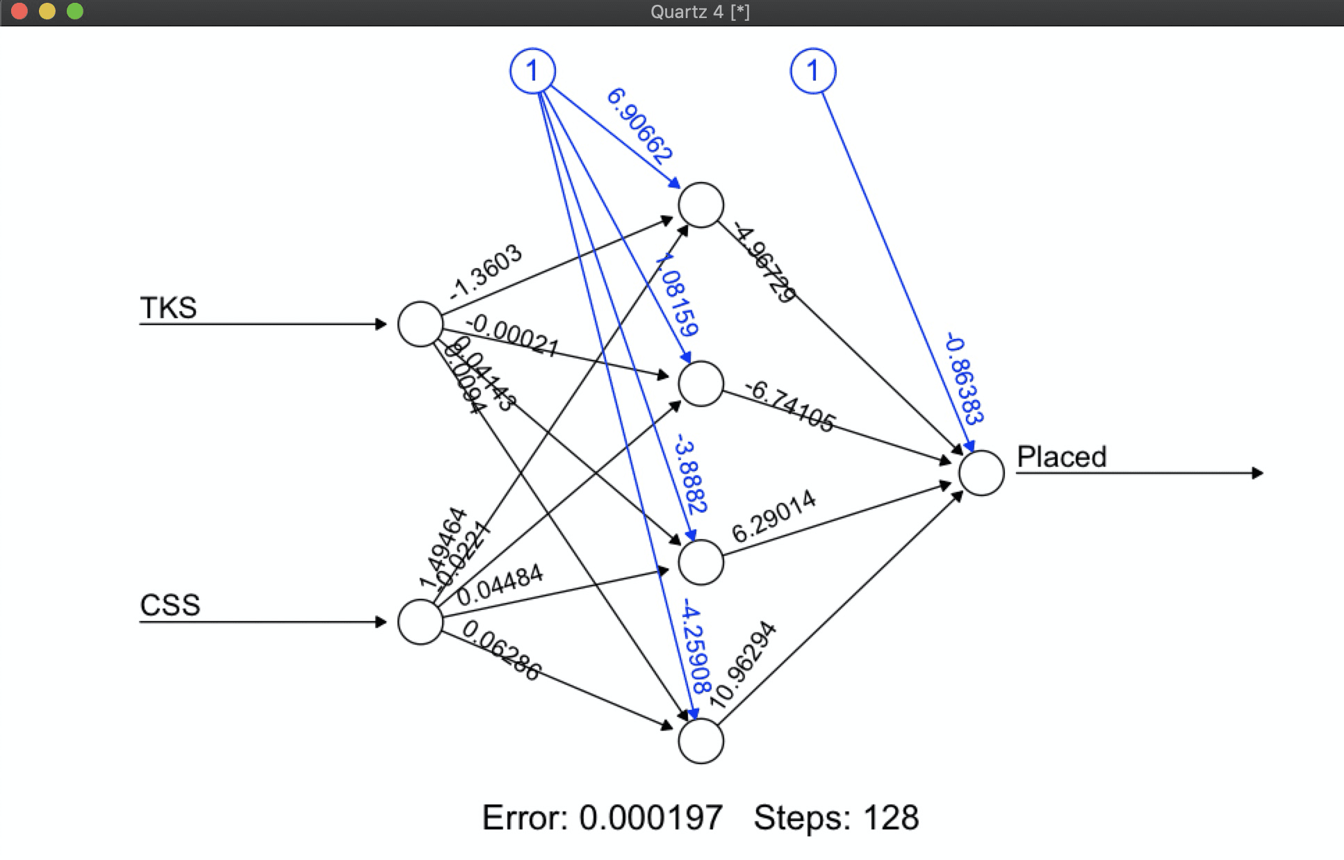
library(neuralnet)

###  Loading Data --- --- --- --- --- --- --- --- --- --- --- --- --- --- ----
# creating train dataset ~~~~~~~~~~~~~~~~~~~~~~~~~~~~~~~~~~~~~~~~~~~~~~~~~~~~~~~
TKS    <- c(20,10,30,20,80,30)     #technical     Knowledge Score -feature
CSS    <- c(90,20,40,50,50,80)     #Communication Knowledge Score -feature
Placed <- c( 1, 0, 0, 0, 1, 1)     #Student Placed                -binary label

trnData <- data.frame(TKS,CSS,Placed)

# creating test dataset ~~~~~~~~~~~~~~~~~~~~~~~~~~~~~~~~~~~~~~~~~~~~~~~~~~~~~~~~
TKS    <- c(30,40,85)
CSS    <- c(85,50,40)

tstData <- data.frame(TKS,CSS)

# Network  --- --- --- --- --- --- --- --- --- --- --- --- --- --- --- --- ----
model <- neuralnet( Placed ~ TKS+CSS, data=trnData, 
                    hidden=4, act.fct ="logistic", linear.output=F)
model %>% plot()

## Prediction using neural network -- --- --- --- --- --- --- --- --- --- ----
pred <- compute(model, tstData)
pred.prob <- pred$net.result

pred <- ifelse(pred.prob>0.5, 1, 0)
pred

     [,1]
[1,]    1
[2,]    0
[3,]    1

classification

# Binary classification
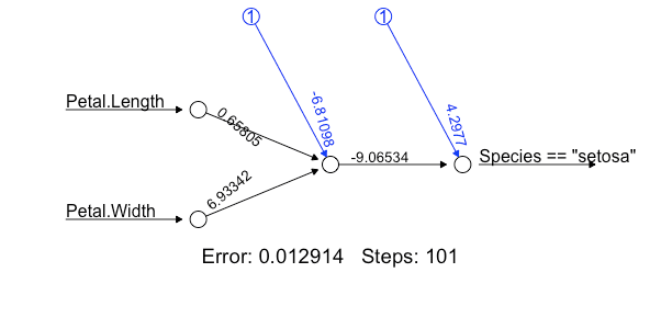
nn <- neuralnet(formula= (Species=="setosa")~ Petal.Length + Petal.Width, 
                data=iris,
                linear.output=FALSE)

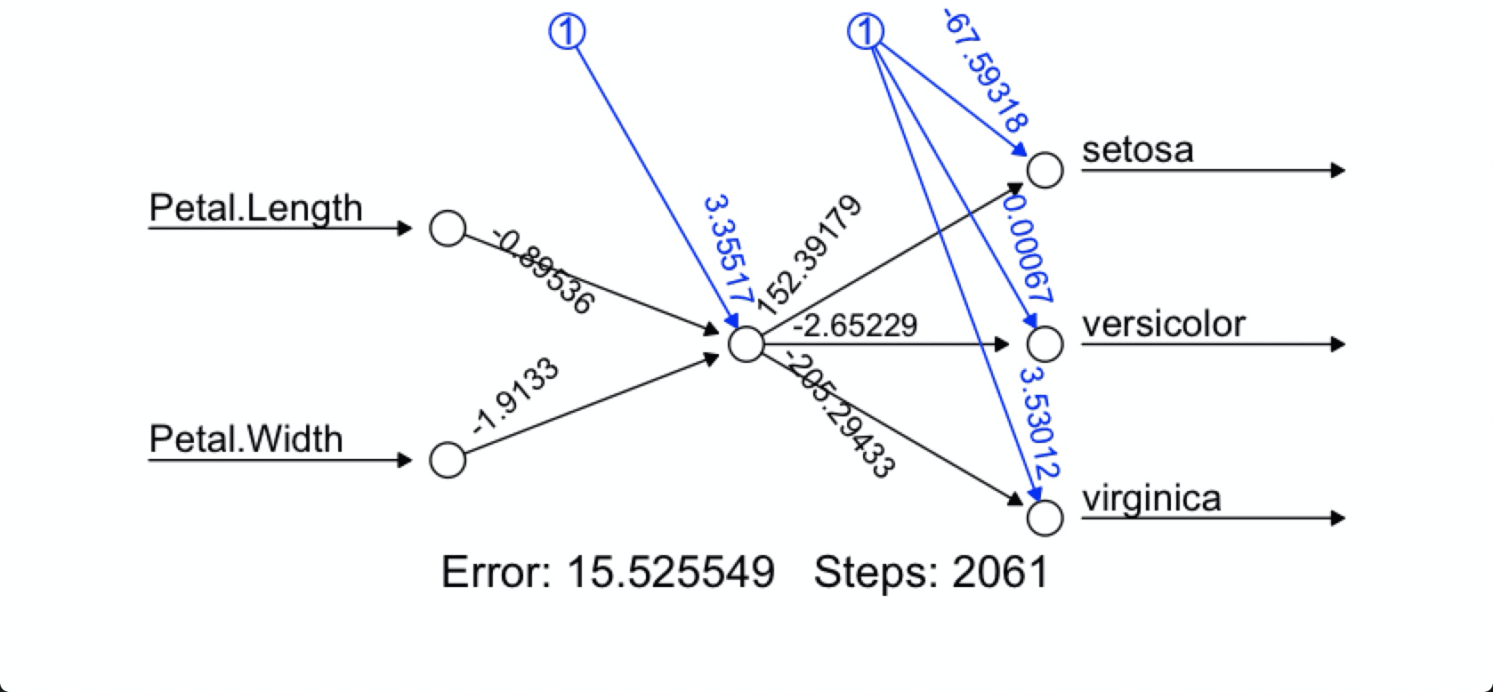
# Multiclass classification
nn <- neuralnet(formula= Species ~ Petal.Length + Petal.Width,
                data=iris,
                linear.output=FALSE)

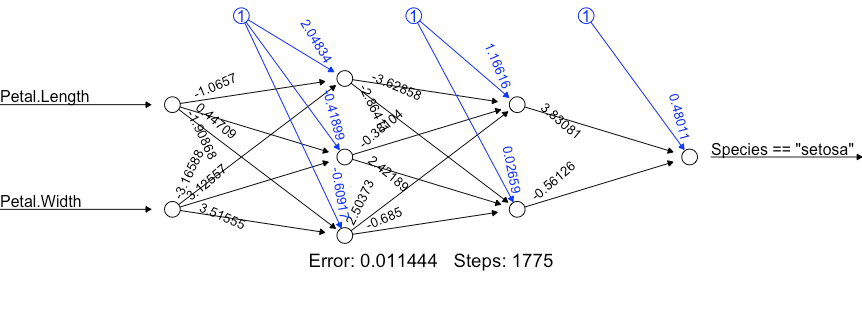
# Custom activation function
softplus <- function(x) log(1 + exp(x))
nn <- neuralnet(formula= (Species=="setosa")~ Petal.Length + Petal.Width, 
                data=iris,
                linear.output=FALSE,
                hidden = c(3, 2), 
                act.fct = softplus)

print(nn)
plot(nn)

library(neuralnet)
library(ggpmisc)
set.seed(2016)

# Load Data ---------------------------------------------------------------
attribute <- as.data.frame(sample(seq(-2,2, length=50), 50, replace=F), ncol=1)
response <- attribute^2
d0 <- cbind(attribute, response)
colnames(d0) <- c("attribute", "response")
d0 %>% head()

# ploting for TURE Value --------------------------------------------------
d0 %>% ggplot(aes(x=attribute, y=response)) + geom_point()

# Neuralnet regression ----------------------------------------------------
fit <- neuralnet(response~attribute, data=d0, hidden=c(3,3), threshold =0.01)
fit %>% summary
fit$net.result

# Predict  ----------------------------------------------------------------
result <- cbind(d0, fit$net.result) %>% as.data.table()
colnames(result) <- c("attribute","response", "Pred")

result %>% ggplot(aes(x=attribute)) + 
    geom_point(aes(y=response)) + geom_point(aes(y=Pred), color="red")
result %>% ggplot(aes(x=response, y=Pred)) + 
    geom_point() + geom_smooth(method="lm", formula=y~x, se=F) + 
    stat_poly_eq(aes(label=..adj.rr.label..), formula=y~x, parse=T)

Resid <- result[, .(response-Pred)]
Resid %>% ggplot(aes(x=1:50, y=V1)) + geom_point()+ 
  geom_smooth(method="lm", formula=y~x, se=F)

library('neuralnet')
library('Metrics')    # for access model
library('ggpmisc')

### Load data ---------------------------------------------------------------
data("Boston", package="MASS")
dd <- Boston %>% data.table()
d1 <- scale(dd) %>% data.table()   # x-mean/sd
keepcolumn <- c("crim","indus","nox","rm","age","dis","tax","ptratio","lstat","medv")
d2 <- d1[ , ..keepcolumn]

# Check NA
d2 %>% map_int( ~ sum(is.na(.)))

# Check Correlation 
d2corr <- cor(d2)
d2melt <- melt(d2corr, varnames=c("x", "y"), value.name="Correlation")
d2melt <- d2melt[order(d2melt$Correlation), ]
d2melt %>% ggplot(aes(x=x, y=y)) + geom_tile(aes(fill=Correlation)) +
  scale_fill_gradient2( 
    low="red", mid="white", high="steelblue",
    guide=guide_colorbar(ticks=F, barheight=10),limits=c(-1, 1)) +
  theme_minimal() + labs(x=NULL, y=NULL)

GGally::ggpairs(d2)
GGally::ggpairs(dd[ , ..keepcolumn])


### Model ---------------------------------------------------------------
set.seed(666)
train <- sample(x=1:dim(d2)[1], size=400, replace=F)

# fit <- neuralnet(formula= medv~crim+indus+nox+rm+age+dis+tax+ptratio+lstat,
#                  data= d2[train, ])
fit <- neuralnet(formula= medv~crim+indus+nox+rm+age+dis+tax+ptratio+lstat,
                 data= d2[train, ],
                 hidden=c(10,12,20),  # No of Neurun for each Hidden layer
                 algorithm= "rprop+", # Resilient backpropagration with backtracking (instead of default 'backprop' with learningrate=0.01)
                 err.fct= "sse",      # Error Function
                 act.fct= "logistic", # Activation Function
                 threshold= 0.1,      # Activation Function threshold
                 linear.output= TRUE  # Output layer neurun, 
      )
#pred <- compute(x=fit, covariate=d2[-train, 1:9])
pred <- predict(fit, newdata=d2[-train, 1:9])

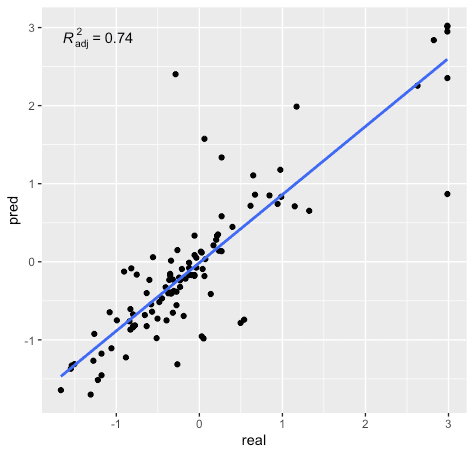
### Assess Model ---------------------------------------------------------------
cor(d2[-train,][[10]] , pred)^2
#0.7458
mse(d2[-train,][[10]] , pred)
#0.2732
rmse(d2[-train,][[10]] , pred)  # sqrt(mse)
#0.5227
RealvsPred <- cbind(d2[-train,][[10]] , pred) %>% data.table()
names(RealvsPred) <- c("real", "pred")
RealvsPred %>% ggplot(aes(x=real, y=pred)) + geom_point() + 
  geom_smooth(method="lm", formula=y~x, se=F) + stat_poly_eq(aes(label=..adj.rr.label..), formula=y~x, parse=T)

library(deepnet)
xx <- d2[train, 1:9] %>% as.matrix()
yy <- d2[train, 10]  %>% as.matrix()

fit <- nn.train(x=xx, y=yy, 
                initW=NULL, initB=NULL,   # initial weights, bias
                hidden=c(10,12,20),
                learningrate= 0.58,       # for Backprop 
                momentum=0.74,            # 경사하강 업데이틍에서 과거 결사들에 대한 가중치 평균 
                learningrate_scale=1,     # 학습률 
                activationfun="sigm",     
                output="linear",
                numepochs=970,
                batchsize=60,
                hidden_dropout=0,
                visible_dropout=0
      )
pred <- nn.predict(fit, x=d2[-train, 1:9])

DNN (Deep Neural Network)

Neural Network

classification

onesixx

Keras

8.0

Keras

tf$keras$callbacks

Keras

Tensorflow 2.x

DNN (Deep Neural Network)

Neural Network

classification

onesixx

Related Posts

Keras

8.0

Keras

tf$keras$callbacks

Keras

Tensorflow 2.x