1D-CNN-HAR
짧은 구간에 대해서 흥미로운 패턴을 인식하고 싶고, location에 상관없을 때 좋다.
2D이미지로 따지자면 고양이가 이미지 상에서 어느 location에 있던지 상관없어야 하니 맞는말인듯 하다.
주식에 대입해보면 어떨까? 아쉽게도 주식은 trend 및 seasonality가 존재하기 때문에 location에 영향을 받는다고 해야할 것 같다. 상승 패턴이라고 하더라도 방금전에 나온것과 한달전에 나온것은 다르기 때문이다.
예제>

80*3 데이터셋에, 크기가 10 (10*3)인 서로다른 100개의 filter를 적용하는 Conv 1st layer 만들고,
같은 작업을 한번더 Conv 2nd layer에서 시행하여, 마지막 ouput은 62 *100 사이즈 행렬.
pooling과 dropout으로 overfitting을 방지하고, 적절한 activation function으로 결과를 만들어 낸다.
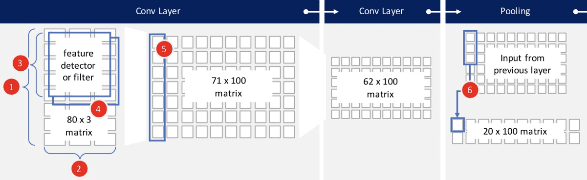
- Height : Network에 넣을 한개의 input데이터셋 length, ex) 80행
- width : Network에 넣을 한개의 input데이터셋 depth, ex) accelerometer센서 x, y, z 3열
- Filter = Feature detector = Sliding window ex) 필터크기 10 * 3 , 각 filter 당 결과 1개
kernel Size : filter의 크기, ex) 10행, filter가 아래로 (80-10+1)=71 만틈 아래쪽으로 슬라이딩 - filters의 종류갯수 ex) 100개의 서로다른 filter , 즉 서로다른 100개의 feature를 뽑아냄.
- Output : 원데이터의 갯수 height 와 kenel Size 에 따라 행의 갯수가 정해지고,
filter의 종률개수만큼의 열갯수가 정해진다.
ex) 1st 출력뉴런은 (80-10+1) * 100 => 기본적인 feature를 학습,
2nd 출력뉴런은 (71 -10+1) *100 => 좀 더 복잡한 feature를 학습 - Max Pooling : (정해진 수만큼 sliding하면서) 그 feature들 중 max value만 취해 대치하고 나머진 버리므로써
학습된 feature의 overfitting을 방지한다. ex> 3행씩, 즉 이전 layer의 66%를 버린다. ouput은 floor(62/3) * 100

– 추가적인 Conv layer 와 추가적인 (Average) pooling
– Dropout : 추가적인 overfitting 방지를 위해, input된 units의 일부(dropout rate만큼)를 임의로 0으로 만든다.
ex) dropout rate = 0.5 50%의 뉴런을 날려, network이 작은 변화에 덜 민감하도록 만듬.
7. Dense : fully connected layer, softmax activation function을 사용하여 6개의 class를 가진 확률분포(Probability districution)를 만든다.
8. Final Ouput : 구하고자 하는 class별로 확률을 만든다.
Human Activity Recognition (HAR)
데이터를 통해 사용자의 activity 유형을 분류 ( “Downstairs”,”Jogging”,”Sitting”,”Standing”,”Upstairs”,”Walking”)
=> HAR (Human Activity Recognition part1, part2)
Data : 스마트폰 accelerometer sensor 데이터, 시간에 따라 등간격으로 측정 , x/y/z 축
WISDM_ar_v1.1_raw.txt github, kaggle
Smartphone-Based Recognition of Human Activities and Postural Transitions Data Set distributed by the University of California, Irvine.
https://blogs.rstudio.com/ai/posts/2018-07-17-activity-detection/
스마트폰의 데이터를 통해 physical activities를 예측하는 것
data: 30명 스마트폰의 accelerometer 와 gyroscope 데이터 (HAPT)
- feature extraction 기법(fast-fourier transform)으로 pre-processed 데이터
- raw data (x, y, z)
### Classifying activity (HAR) ~~~
# https://blogs.rstudio.com/ai/posts/2018-07-17-activity-detection/
source(file.path(getwd(),"../00.global_dl.R"))
library(knitr)
library(rmarkdown)
###### ~~~~~~~~~~~~~~~~~~~~~~~~~~~~~~~~~~~~~~~~~~~~~~~~~~~~~~~~~~~~~~~~~~~~~~~~~
## 10. Load data ----
######~~~~~~~~~~~~~~~~~~~~~~~~~~~~~~~~~~~~~~~~~~~~~~~~~~~~~~~~~~~~~~~~~~~~~~~~~~
### ` === Raw Data -------------------------------------------------------------
# http://archive.ics.uci.edu/ml/datasets/Smartphone-Based+Recognition+of+Human+Activities+and+Postural+Transitions
URL="http://archive.ics.uci.edu/ml/machine-learning-databases/00341/HAPT%20Data%20Set.zip"
temp <- tempfile()
download.file(URL, temp)
unzip(temp, exdir=file.path(DATA_PATH,"HAPT"))
unlink(temp)
rm(temp, URL)
### ` ` * Load -----------------------------------------------------------------
activityLabels <- fread(file.path(DATA_PATH,"HAPT","activity_labels.txt"),
col.names=c("number", "label"))
infoLabels <- fread(file.path(DATA_PATH,"HAPT","RawData","labels.txt"),
col.names = c("experiment", "userId", "activity", "startPos", "endPos"))
dataFiles <- list.files(file.path(DATA_PATH,"HAPT","RawData"), pattern=".*[0-9].txt")
#dataFiles %>% glimpse()
### acc/gyro _ exp1-61 _ user1-30 . txt
fileInfo <- data.table(filePath = dataFiles) %>% # filter(filePath != "labels.txt") %>%
separate(filePath, sep = '_', into = c("type", "experiment", "userId"), remove=F) %>%
mutate( experiment = str_remove(experiment, "exp"),
userId = str_remove_all(userId, "user|\\\\.txt") ) %>%
select(experiment,userId,type,filePath) %>%
spread(key=type, value=filePath)
fileInfo %>% head()
fileInfo %>% glimpse()
### ` ` * Reading and gathering data -------------------------------------------
# Read contents of single file to a dataframe with accelerometer and gyro data.
# fread("/Users/onesixx/DATA/CNN/HAPT/RawData/acc_exp01_user01.txt", col.names=c("a_x","a_y","a_z"))
readInData <- function(experiment, userId){
## : read data from files----
genFilePath <- function(type){
## : get path ----
file.path(DATA_PATH,"HAPT","RawData",str_c(type,"_exp",experiment,"_user",userId,".txt"))
}
bind_cols(
fread(genFilePath("acc"), col.names=c("a_x","a_y","a_z")),
fread(genFilePath("gyro"), col.names=c("g_x","g_y","g_z"))
)
}
# Read a given file and get the observations contained along with their classes.
loadFileData <- function(curExperiment, curUserId) {
## : load data from files----
# curExperiment="01"; curUserId="01"
# load sensor data from file into data.frame
allData <- readInData(curExperiment, curUserId)
# get observation locations in this file from labels dataframe
label_byExperimentUserId <- infoLabels %>%
filter(userId ==as.integer(curUserId),
experiment==as.integer(curExperiment))
# extract observations as dataframes and save as a column in dataframe.
label_byExperimentUserId %>%
mutate(data=map2(startPos, endPos, function(startPos, endPos){ # extractObservation
allData[startPos:endPos,]
}) ) %>%
select(-startPos, -endPos)
}
# scan through all experiment and userId combos and gather data into a dataframe.
allObservations <- map2_df(fileInfo$experiment, fileInfo$userId, loadFileData) %>%
right_join(activityLabels, by= c("activity"="number")) %>%
rename(activityName=label)
# cache work.
#ifelse(dir.exists(file.path(DATA_PATH,"PreProcess")), cat("OK","\
"), dir.create(file.path(DATA_PATH,"PreProcess")))
#write_fst(allObservations, file.path(DATA_PATH,"allObservations.fst"))
saveRDS(allObservations, file.path(DATA_PATH,"HAPT_obs.rds"))
allObservations %>% dim()
rm(allObservations)
## ` ` * Read RDS again ----
#allObservations <- read_fst(file.path(DATA_PATH,"allObservations.fst"))
allObservations <- readRDS(file.path(DATA_PATH,"HAPT_obs.rds"))
allObservations %>% head(20)
# allObservations %>%
# filter(activityName=="WALKING_UPSTAIRS") %>%
# mutate(recording_length=map_int(data, nrow)) %>%
# select(activityName, recording_length) %>%
# ggplot(aes(x=recording_length, y=activityName)) +
# geom_density_ridges(alpha=0.8)
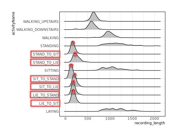
allObservations %>%
mutate(recording_length=map_int(data, nrow)) %>%
ggplot(aes(x=recording_length, y=activityName)) +
ggridges::geom_density_ridges(alpha=0.8)
# activity간에 recording_length에 차이가 있다.
# => 가장 Length가 긴 activity에 맞춰 padding-zeros할 필요
unique(allObservations$activityName)
### ` ` * Filtering activities ----
desiredActivities <- c(
"STAND_TO_SIT", "SIT_TO_STAND", "SIT_TO_LIE",
"LIE_TO_SIT", "STAND_TO_LIE", "LIE_TO_STAND"
)
filteredObservations <- allObservations %>%
filter(activityName %in% desiredActivities) %>%
mutate(observationId=1:n())
filteredObservations
#unique(filteredObservations$activityName)
### ` ` * Training/testing split ----
set.seed(42)
## randomly choose 24 for training (80% of 30 individuals)
## set the rest of the users to the testing set
## get all users : 30명
userIds <- filteredObservations$userId %>% unique()
trainIds <- userIds %>% sample(size=24)
testIds <- userIds %>% setdiff(trainIds)
## filter data.
trainData <- filteredObservations %>% filter(userId %in% trainIds)
testData <- filteredObservations %>% filter(userId %in% testIds)
### ` === EDA ------------------------------------------------------------------
unpackedObs <- 1:nrow(trainData) %>%
map_df(function(rowNum){
#rowNum=1
dataRow <- trainData[rowNum, ]
dataRow$data[[1]] %>%
mutate(activityName =dataRow$activityName,
observationId=dataRow$observationId,
time = 1:n())
}) %>%
#gather(reading, value, -time, -activityName, -observationId) %>%
gather(key=reading, value=value, a_x,a_y,a_z, g_x,g_y,g_z) %>%
separate(col=reading, into=c("type", "direction"), sep="_") %>%
mutate(type=ifelse(type=="a", "acceleration", "gyro")) %>% as.data.table()
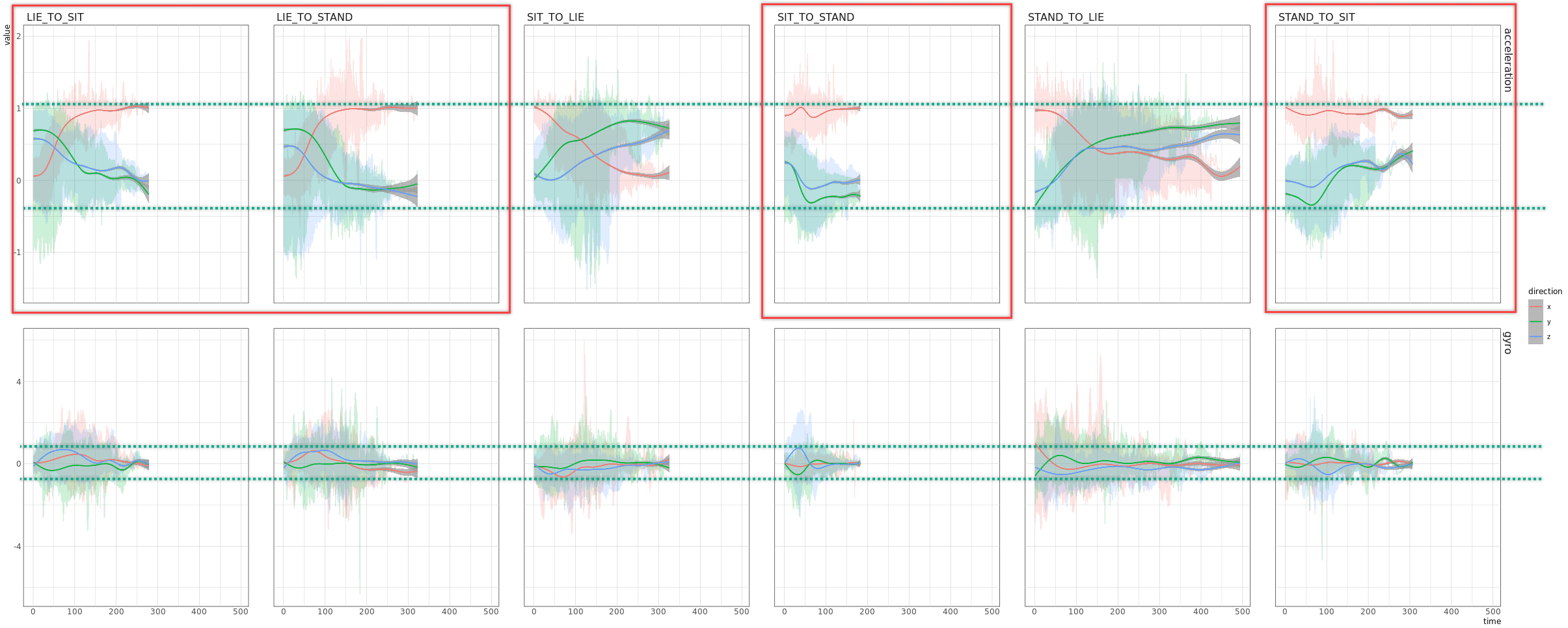
unpackedObs %>% #filter(type=="acceleration") %>%
ggplot(aes(x=time, y=value, color=direction)) +
geom_line(alpha=.2) +
geom_smooth(size=.5, alpha=.7) +
geom_smooth(se=F, alpha=.7, size=.5) +
facet_grid(type ~ activityName)
unpackedObs[activityName=="STAND_TO_SIT" & observationId=="1" & type=="acceleration", ]
### ` === Preprocess : Normalize / rescale / ----------------------------------
### ` === INPUT LAYER ----------------------------------------------------------
# convert list of obs to matrices
# pad all obs
# turn into a 3D tensor
## ` ` * Padding(truncate) observations ----
# truncate long length obs (outlier)
padSize <- trainData$data %>% map_int(nrow) %>%
quantile(p=.98) %>% ceiling()
dataset <- data.table(trainData$data %>% map_int(nrow))
dataset%>%
ggplot(aes(V1)) +
geom_density() + #(aes(y=..density..)))
geom_vline(aes(xintercept= quantile(dataset$V1, prob=.98)), color="red", size=.6) +
scale_y_continuous(expand=c(0, NA))
convertToTensor <- function(myList) {
# : keras::pad_sequences() ----
# myList = trainData$data[1]
myList %>% map(as.matrix) %>%
pad_sequences(maxlen=padSize)
}
# convertToTensor <- . %>% map(as.matrix) %>%
# pad_sequences(maxlen=padSize)
trainObs <- trainData$data %>% convertToTensor()
testObs <- testData$data %>% convertToTensor()
# trainData$data %>% length [1] 290 of list
# trainObs %>% dim [1] 290 320 6 of array
# trainData %>% mutate(nn=map_int(data, nrow)) %>% arrange(desc(nn))
# tt <- trainData[observationId==281, data] %>% convertToTensor()
tt <- trainObs[281,,]
# tt0 <- trainData$data %>% map(function(x){ x[x!=0]<-1; x })
# ttObs <- tt0 %>% convertToTensor()
# tt <- ttObs[281,,]
reshape2::melt(tt) %>%
ggplot(aes(Var2, Var1, fill=value)) + geom_tile(color="white") +
scale_fill_gradient2(limit=c(-1,1), midpoint=0, name="",
low="blue",mid="white",high="red")
# keras::pad_sequences(sequences, maxlen=NULL, dtype="int32",
# padding="pre", truncating="pre", value=0
# )
# 길이가 다른 sequences를 같은길이로 맞출때, 2,3차원 모두 가능
trainObs %>% dim() # 290 maxLength 6 (, , )
testObs %>% dim() # 68 333 6
## ` ` One-hot encoding ----
#filteredObservations$activity %>% unique() %>% sort()
oneHotClasses <- . %>% {. -7} %>% # bring integers down to 0-6 from 7-12
to_categorical() # One-hot encode
trainY <- trainData$activity %>% oneHotClasses()
testY <- testData$activity %>% oneHotClasses()
###### ~~~~~~~~~~~~~~~~~~~~~~~~~~~~~~~~~~~~~~~~~~~~~~~~~~~~~~~~~~~~~~~~~~~~~~~~~
### 20. Train the model ----
###### ~~~~~~~~~~~~~~~~~~~~~~~~~~~~~~~~~~~~~~~~~~~~~~~~~~~~~~~~~~~~~~~~~~~~~~~~~
### ` === Build/Reshape/complie the model --------------------------------------
input_shape <- dim(trainObs)[-1]
num_classes <- dim(trainY)[2]
filters <- 24 # number of convolutional filters to learn
kernel_size <- 8 # how many time-steps each conv layer sees.
dense_size <- 48 # size of our penultimate dense layer.
# Initialize model
model <- keras_model_sequential()
model %>%
layer_conv_1d(input_shape=input_shape, filters=filters, kernel_size=kernel_size,
padding="valid", activation="relu") %>%
layer_batch_normalization() %>%
layer_spatial_dropout_1d(0.15) %>%
layer_conv_1d(filters = filters/2, kernel_size = kernel_size,
activation = "relu") %>%
# Apply average pooling:
layer_global_average_pooling_1d() %>%
layer_batch_normalization() %>%
layer_dropout(0.2) %>%
layer_dense(dense_size, activation="relu") %>%
layer_batch_normalization() %>%
layer_dropout(0.25) %>%
layer_dense(num_classes, activation="softmax", name="dense_output")
summary(model)
### ` === Train(fitting) the model : history, summary --------------------------
model %>% compile(
loss = "categorical_crossentropy",
optimizer = "rmsprop",
metrics = "accuracy"
)
trainHistory <- model %>% fit(x=trainObs, y=trainY,
epochs=350,
validation_data=list(testObs, testY),
callbacks=list(
callback_model_checkpoint("best_model.h5", save_best_only=T)
)
)
trainHistory
###### ~~~~~~~~~~~~~~~~~~~~~~~~~~~~~~~~~~~~~~~~~~~~~~~~~~~~~~~~~~~~~~~~~~~~~~~~~
### 30. Evaluation ----
###### ~~~~~~~~~~~~~~~~~~~~~~~~~~~~~~~~~~~~~~~~~~~~~~~~~~~~~~~~~~~~~~~~~~~~~~~~~
### ` === Evaluate accuracy ----------------------------------------------------
# dataframe to get labels onto one-hot encoded prediction columns
oneHotToLabel <- activityLabels %>% mutate(number=number-7) %>% filter(number>=0) %>%
mutate(class=paste0("V",number+1)) %>%
select(-number)
# Load our best model checkpoint
bestModel <- load_model_hdf5("best_model.h5")
tidyPredictionProbs <- bestModel %>% predict(testObs) %>% data.table() %>%
mutate(obs=1:n()) %>%
gather(class, prob, -obs) %>%
right_join(oneHotToLabel, by = "class")
### ` === Improve the model ----------------------------------------------------
###### ~~~~~~~~~~~~~~~~~~~~~~~~~~~~~~~~~~~~~~~~~~~~~~~~~~~~~~~~~~~~~~~~~~~~~~~~~
### 40. Make predictions ----
###### ~~~~~~~~~~~~~~~~~~~~~~~~~~~~~~~~~~~~~~~~~~~~~~~~~~~~~~~~~~~~~~~~~~~~~~~~~
### ` === explain Model --------------------------------------------------------
### ` === NEW DATA predictions -------------------------------------------------
predictionPerformance <- tidyPredictionProbs %>%
group_by(obs) %>%
summarise(
highestProb = max(prob),
predicted = label[prob == highestProb]
) %>%
mutate(
truth = testData$activityName,
correct = truth == predicted
)
predictionPerformance %>% paged_table()
predictionPerformance
predictionPerformance %>% mutate(result=ifelse(correct,'Correct','Incorrect')) %>%
ggplot(aes(highestProb)) +
geom_histogram(binwidth=.01) +
geom_rug(alpha=.5) +
facet_grid(result~.) +
ggtitle("Probabilities associated with prediction by correctness")
predictionPerformance %>%
group_by(truth, predicted) %>% summarise(count=n()) %>%
mutate(good= (truth==predicted)) %>%
ggplot(aes(x=truth, y=predicted)) +
geom_point(aes(size=count, color=good)) +
geom_text(aes(label=count), hjust=0, vjust=0, nudge_x=.1, nudge_y=.1) +
guides(color=F, size=F)
keras::pad_sequence()
- maxlen 인자로 문장의 길이를 맞춰줍니다.
예를 들어 120으로 지정했다면 120보다 짧은 문장은 0으로 채워서 120단어로 맞춰주고 120보다 긴 문장은 120단어까지만 잘라냅니다. - (num_samples, num_timesteps)으로 2차원의 numpy 배열로 만들어줍니다.
maxlen을 120으로 지정하였다면, num_timesteps도 120이 됩니다.
> library(keras)
> X = matrix(c(1.01528, -2.141667, 3.0597222,
+              1.02083, -1.999999, 0.0555556,
+              1.02778, -0.173611, 0.0694444,
+             -1,        0,        1         ), nrow=4, ncol=3, byrow=T)
> X
         [,1]      [,2]      [,3]
[1,]  1.01528 -2.141667 3.0597222
[2,]  1.02083 -1.999999 0.0555556
[3,]  1.02778 -0.173611 0.0694444
[4,] -1.00000  0.000000 1.0000000
> X %>% pad_sequences()
     [,1] [,2] [,3]
[1,]    1   -2    3
[2,]    1   -1    0
[3,]    1    0    0
[4,]   -1    0    1
> X %>% pad_sequences(maxlen=6)
     [,1] [,2] [,3] [,4] [,5] [,6]
[1,]    0    0    0    1   -2    3
[2,]    0    0    0    1   -1    0
[3,]    0    0    0    1    0    0
[4,]    0    0    0   -1    0    1


> X = list(matrix(c(1.01528, -2.141667, 3.0597222,
+              1.02083, -1.999999, 0.0555556,
+              1.02778, -0.173611, 0.0694444,
+              -1,        0,        1         ), nrow=4, ncol=3, byrow=T))
> X
[[1]]
         [,1]      [,2]      [,3]
[1,]  1.01528 -2.141667 3.0597222
[2,]  1.02083 -1.999999 0.0555556
[3,]  1.02778 -0.173611 0.0694444
[4,] -1.00000  0.000000 1.0000000

> X %>% pad_sequences()
, , 1
     [,1] [,2] [,3] [,4]
[1,]    1    1    1   -1
, , 2
     [,1] [,2] [,3] [,4]
[1,]   -2   -1    0    0
, , 3
     [,1] [,2] [,3] [,4]
[1,]    3    0    0    1

> X %>% pad_sequences(maxlen=6)
, , 1
     [,1] [,2] [,3] [,4] [,5] [,6]
[1,]    0    0    1    1    1   -1
, , 2
     [,1] [,2] [,3] [,4] [,5] [,6]
[1,]    0    0   -2   -1    0    0
, , 3
     [,1] [,2] [,3] [,4] [,5] [,6]
[1,]    0    0    3    0    0    1
> summary(model)
Model: "sequential_2"
_______________________________________________________________________________
Layer (type)                                        Output Shape       Param #
===============================================================================
conv1d (Conv1D)                                     (None, 313, 24)     1176
_______________________________________________________________________________
batch_normalization (BatchNormalization)            (None, 313, 24)       96
_______________________________________________________________________________
spatial_dropout1d (SpatialDropout1D)                (None, 313, 24)        0
______________________________________________________________________________
conv1d_1 (Conv1D)                                   (None, 306, 12)     2316
_______________________________________________________________________________
global_average_pooling1d (GlobalAveragePooling1D)   (None, 12)             0
______________________________________________________________________________
batch_normalization_1 (BatchNormalization)          (None, 12)            48
_______________________________________________________________________________
dropout (Dropout)                                   (None, 12)             0
_______________________________________________________________________________
dense (Dense)                                       (None, 48)           624
_______________________________________________________________________________
batch_normalization_2 (BatchNormalization)          (None, 48)           192
_______________________________________________________________________________
dropout_1 (Dropout)                                 (None, 48)             0
_______________________________________________________________________________
dense_output (Dense)                                (None, 6)            294
===============================================================================
Total params: 4,746
Trainable params: 4,578
Non-trainable params: 168
______________________________________________________________________________
Links and References
https://keras.io/guides/sequential_model/
- Keras documentation for 1D convolutional neural networks
- Keras examples for 1D convolutional neural networks
- A good article with an introduction to 1D CNNs for natural language processing problems
### Classifying activity (HAR) ~~~
# https://blogs.rstudio.com/ai/posts/2018-07-17-activity-detection/
source(file.path(getwd(),"../00.global_dl.R"))

library(knitr)
library(rmarkdown)

###### ~~~~~~~~~~~~~~~~~~~~~~~~~~~~~~~~~~~~~~~~~~~~~~~~~~~~~~~~~~~~~~~~~~~~~~~~~
## 10. Load data ----
######~~~~~~~~~~~~~~~~~~~~~~~~~~~~~~~~~~~~~~~~~~~~~~~~~~~~~~~~~~~~~~~~~~~~~~~~~~
### ` === Raw Data -------------------------------------------------------------
# http://archive.ics.uci.edu/ml/datasets/Smartphone-Based+Recognition+of+Human+Activities+and+Postural+Transitions
URL="http://archive.ics.uci.edu/ml/machine-learning-databases/00341/HAPT%20Data%20Set.zip"
temp <- tempfile()
download.file(URL, temp)
unzip(temp, exdir=file.path(DATA_PATH,"HAPT"))
unlink(temp)

rm(temp, URL)

### ` ` * Load -----------------------------------------------------------------
activityLabels <- fread(file.path(DATA_PATH,"HAPT","activity_labels.txt"),
                        col.names=c("number", "label"))

infoLabels <- fread(file.path(DATA_PATH,"HAPT","RawData","labels.txt"),
                    col.names = c("experiment", "userId", "activity", "startPos", "endPos"))

dataFiles <- list.files(file.path(DATA_PATH,"HAPT","RawData"), pattern=".*[0-9].txt")
#dataFiles %>% glimpse()
###  acc/gyro _ exp1-61 _ user1-30 . txt

fileInfo <- data.table(filePath = dataFiles) %>%  #  filter(filePath != "labels.txt") %>%
  separate(filePath, sep = '_',  into = c("type", "experiment", "userId"), remove=F) %>%
  mutate( experiment = str_remove(experiment, "exp"),
          userId     = str_remove_all(userId, "user|\\\\.txt") ) %>%
  select(experiment,userId,type,filePath) %>%
  spread(key=type, value=filePath)

fileInfo %>% head()
fileInfo %>% glimpse()

### ` ` * Reading and gathering data -------------------------------------------
# Read contents of single file to a dataframe with accelerometer and gyro data.
# fread("/Users/onesixx/DATA/CNN/HAPT/RawData/acc_exp01_user01.txt", col.names=c("a_x","a_y","a_z"))

readInData <- function(experiment, userId){
  ## : read data from files----
  genFilePath <- function(type){
    ## : get path ----
    file.path(DATA_PATH,"HAPT","RawData",str_c(type,"_exp",experiment,"_user",userId,".txt"))
  }
  bind_cols(
    fread(genFilePath("acc"),  col.names=c("a_x","a_y","a_z")),
    fread(genFilePath("gyro"), col.names=c("g_x","g_y","g_z"))
  )
}
# Read a given file and get the observations contained along with their classes.
loadFileData <- function(curExperiment, curUserId) {
  ## : load data from files----
  # curExperiment="01"; curUserId="01"
  # load sensor data from file into data.frame
  allData <- readInData(curExperiment, curUserId)

  # get observation locations in this file from labels dataframe
  label_byExperimentUserId <- infoLabels %>%
    filter(userId    ==as.integer(curUserId),
           experiment==as.integer(curExperiment))
  # extract observations as dataframes and save as a column in dataframe.
  label_byExperimentUserId %>%
    mutate(data=map2(startPos, endPos, function(startPos, endPos){ # extractObservation
      allData[startPos:endPos,]
    }) ) %>%
    select(-startPos, -endPos)
}

# scan through all experiment and userId combos and gather data into a dataframe.
allObservations <- map2_df(fileInfo$experiment, fileInfo$userId, loadFileData) %>%
  right_join(activityLabels, by= c("activity"="number")) %>%
  rename(activityName=label)

# cache work.
#ifelse(dir.exists(file.path(DATA_PATH,"PreProcess")), cat("OK","\
"), dir.create(file.path(DATA_PATH,"PreProcess")))
#write_fst(allObservations, file.path(DATA_PATH,"allObservations.fst"))
saveRDS(allObservations, file.path(DATA_PATH,"HAPT_obs.rds"))
allObservations %>% dim()
rm(allObservations)


## ` ` * Read RDS again ----
#allObservations <- read_fst(file.path(DATA_PATH,"allObservations.fst"))
allObservations <- readRDS(file.path(DATA_PATH,"HAPT_obs.rds"))
allObservations %>% head(20)

# allObservations %>%
#   filter(activityName=="WALKING_UPSTAIRS") %>%
#   mutate(recording_length=map_int(data, nrow)) %>%
#   select(activityName, recording_length) %>%
#   ggplot(aes(x=recording_length, y=activityName)) +
#   geom_density_ridges(alpha=0.8)


allObservations %>%
  mutate(recording_length=map_int(data, nrow)) %>%
  ggplot(aes(x=recording_length, y=activityName)) +
  ggridges::geom_density_ridges(alpha=0.8)

# activity간에 recording_length에 차이가 있다.
# => 가장 Length가 긴 activity에 맞춰 padding-zeros할 필요
unique(allObservations$activityName)

### ` ` * Filtering activities ----
desiredActivities <- c(
  "STAND_TO_SIT", "SIT_TO_STAND", "SIT_TO_LIE",
  "LIE_TO_SIT",   "STAND_TO_LIE", "LIE_TO_STAND"
)

filteredObservations <- allObservations %>%
  filter(activityName %in% desiredActivities) %>%
  mutate(observationId=1:n())

filteredObservations
#unique(filteredObservations$activityName)


### ` ` * Training/testing split ----
set.seed(42)
## randomly choose 24 for training (80% of 30 individuals)
## set the rest of the users to the testing set
## get all users : 30명
userIds  <- filteredObservations$userId %>% unique()
trainIds <- userIds %>% sample(size=24)
testIds  <- userIds %>% setdiff(trainIds)

## filter data.
trainData <- filteredObservations %>% filter(userId %in% trainIds)
testData  <- filteredObservations %>% filter(userId %in% testIds)

### ` === EDA ------------------------------------------------------------------
unpackedObs <- 1:nrow(trainData) %>%
  map_df(function(rowNum){
    #rowNum=1
    dataRow <- trainData[rowNum, ]

    dataRow$data[[1]] %>%
      mutate(activityName =dataRow$activityName,
             observationId=dataRow$observationId,
             time         = 1:n())
  }) %>%
  #gather(reading, value, -time, -activityName, -observationId) %>%
  gather(key=reading, value=value, a_x,a_y,a_z, g_x,g_y,g_z) %>%
  separate(col=reading, into=c("type", "direction"), sep="_") %>%
  mutate(type=ifelse(type=="a", "acceleration", "gyro")) %>% as.data.table()

unpackedObs %>% #filter(type=="acceleration") %>%
  ggplot(aes(x=time, y=value, color=direction)) +
  geom_line(alpha=.2) +
  geom_smooth(size=.5, alpha=.7) +
  geom_smooth(se=F, alpha=.7, size=.5) +
  facet_grid(type ~ activityName)

unpackedObs[activityName=="STAND_TO_SIT" & observationId=="1" & type=="acceleration", ]

### ` === Preprocess : Normalize / rescale /  ----------------------------------
### ` === INPUT LAYER ----------------------------------------------------------
# convert list of obs to matrices
# pad all obs
# turn into a 3D tensor

## ` ` * Padding(truncate) observations ----
# truncate long length obs (outlier)
padSize <- trainData$data %>% map_int(nrow) %>%
              quantile(p=.98) %>% ceiling()

dataset <- data.table(trainData$data %>% map_int(nrow))
dataset%>%
  ggplot(aes(V1)) +
  geom_density() + #(aes(y=..density..)))
  geom_vline(aes(xintercept= quantile(dataset$V1, prob=.98)), color="red", size=.6) +
  scale_y_continuous(expand=c(0, NA))

convertToTensor <- function(myList) {
  # : keras::pad_sequences() ----
  # myList = trainData$data[1]
  myList %>% map(as.matrix) %>%
    pad_sequences(maxlen=padSize)
}
# convertToTensor <- . %>% map(as.matrix) %>%
#                       pad_sequences(maxlen=padSize)

trainObs <- trainData$data %>% convertToTensor()
testObs  <- testData$data  %>% convertToTensor()

# trainData$data %>% length      [1] 290          of list
# trainObs %>% dim               [1] 290 320   6  of array
# trainData %>% mutate(nn=map_int(data, nrow)) %>% arrange(desc(nn))
# tt <- trainData[observationId==281, data] %>% convertToTensor()
tt <- trainObs[281,,]
# tt0 <- trainData$data %>% map(function(x){ x[x!=0]<-1;  x })
# ttObs <- tt0 %>% convertToTensor()
# tt <- ttObs[281,,]
reshape2::melt(tt) %>%
  ggplot(aes(Var2, Var1, fill=value)) + geom_tile(color="white") +
  scale_fill_gradient2(limit=c(-1,1), midpoint=0, name="",
                       low="blue",mid="white",high="red")

# keras::pad_sequences(sequences, maxlen=NULL, dtype="int32",
#   padding="pre", truncating="pre", value=0
# )
# 길이가 다른 sequences를 같은길이로 맞출때, 2,3차원 모두 가능

trainObs %>% dim()  # 290 maxLength 6 (, , )
testObs  %>% dim()  #  68 333       6

## ` ` One-hot encoding ----
#filteredObservations$activity %>% unique() %>% sort()
oneHotClasses <- . %>% {. -7} %>%   # bring integers down to 0-6 from 7-12
                    to_categorical()   # One-hot encode

trainY <- trainData$activity %>% oneHotClasses()
testY  <- testData$activity  %>% oneHotClasses()

###### ~~~~~~~~~~~~~~~~~~~~~~~~~~~~~~~~~~~~~~~~~~~~~~~~~~~~~~~~~~~~~~~~~~~~~~~~~
### 20. Train the model ----
###### ~~~~~~~~~~~~~~~~~~~~~~~~~~~~~~~~~~~~~~~~~~~~~~~~~~~~~~~~~~~~~~~~~~~~~~~~~
### ` === Build/Reshape/complie the model --------------------------------------
input_shape <- dim(trainObs)[-1]
num_classes <- dim(trainY)[2]

filters <- 24     # number of convolutional filters to learn
kernel_size <- 8  # how many time-steps each conv layer sees.
dense_size <- 48  # size of our penultimate dense layer.

# Initialize model
model <- keras_model_sequential()
model %>%
  layer_conv_1d(input_shape=input_shape, filters=filters, kernel_size=kernel_size,
                padding="valid",  activation="relu") %>%
  layer_batch_normalization() %>%
  layer_spatial_dropout_1d(0.15) %>%
  layer_conv_1d(filters = filters/2, kernel_size = kernel_size,
                activation = "relu") %>%
  # Apply average pooling:
  layer_global_average_pooling_1d() %>%
  layer_batch_normalization() %>%
  layer_dropout(0.2) %>%
  layer_dense(dense_size, activation="relu") %>%
  layer_batch_normalization() %>%
  layer_dropout(0.25) %>%
  layer_dense(num_classes, activation="softmax", name="dense_output")

summary(model)
### ` === Train(fitting) the model : history, summary --------------------------

model %>% compile(
  loss = "categorical_crossentropy",
  optimizer = "rmsprop",
  metrics = "accuracy"
)

trainHistory <- model %>% fit(x=trainObs, y=trainY,
                              epochs=350,
                              validation_data=list(testObs, testY),
                              callbacks=list(
                                callback_model_checkpoint("best_model.h5", save_best_only=T)
                              )
                            )
trainHistory
###### ~~~~~~~~~~~~~~~~~~~~~~~~~~~~~~~~~~~~~~~~~~~~~~~~~~~~~~~~~~~~~~~~~~~~~~~~~
### 30. Evaluation ----
###### ~~~~~~~~~~~~~~~~~~~~~~~~~~~~~~~~~~~~~~~~~~~~~~~~~~~~~~~~~~~~~~~~~~~~~~~~~
### ` === Evaluate accuracy ----------------------------------------------------
# dataframe to get labels onto one-hot encoded prediction columns
oneHotToLabel <- activityLabels %>% mutate(number=number-7) %>% filter(number>=0) %>%
                   mutate(class=paste0("V",number+1)) %>%
                   select(-number)

# Load our best model checkpoint
bestModel <- load_model_hdf5("best_model.h5")

tidyPredictionProbs <- bestModel %>% predict(testObs) %>% data.table() %>%
                        mutate(obs=1:n()) %>%
                        gather(class, prob, -obs) %>%
                        right_join(oneHotToLabel, by = "class")

### ` === Improve the model ----------------------------------------------------

###### ~~~~~~~~~~~~~~~~~~~~~~~~~~~~~~~~~~~~~~~~~~~~~~~~~~~~~~~~~~~~~~~~~~~~~~~~~
### 40. Make predictions ----
###### ~~~~~~~~~~~~~~~~~~~~~~~~~~~~~~~~~~~~~~~~~~~~~~~~~~~~~~~~~~~~~~~~~~~~~~~~~
### ` === explain Model --------------------------------------------------------
### ` === NEW DATA predictions -------------------------------------------------

predictionPerformance <- tidyPredictionProbs %>%
  group_by(obs) %>%
  summarise(
    highestProb = max(prob),
    predicted = label[prob == highestProb]
  ) %>%
  mutate(
    truth = testData$activityName,
    correct = truth == predicted
  )

predictionPerformance %>% paged_table()
predictionPerformance

predictionPerformance %>% mutate(result=ifelse(correct,'Correct','Incorrect')) %>%
  ggplot(aes(highestProb)) +
    geom_histogram(binwidth=.01) +
    geom_rug(alpha=.5) +
    facet_grid(result~.) +
    ggtitle("Probabilities associated with prediction by correctness")


predictionPerformance %>%
  group_by(truth, predicted) %>% summarise(count=n()) %>%
  mutate(good= (truth==predicted)) %>%
  ggplot(aes(x=truth,  y=predicted)) +
    geom_point(aes(size=count, color=good)) +
    geom_text(aes(label=count), hjust=0, vjust=0, nudge_x=.1, nudge_y=.1) +
    guides(color=F, size=F)
