ISLR :: 8.3 Lab: Decision Trees :: 8.3.3 Bagging and Random Forests
http://www.rmdk.ca/boosting_forests_bagging.html
8.3.3 Bagging and Random Forests
DATA
: Boston Medv (주택의 가격 변수)에 대한여러 요건들(13개 변수)간의 관계 분석
####################################################################
# Boston DATA-set
library(MASS)
data("Boston")

set.seed(1)
train <- sample(1:nrow(Boston), nrow(Boston)/2)
boston.train <- Boston[ train, ]
boston.test  <- Boston[-train, ]
'data.frame':	506 obs. of  14 variables:
 $ crim   : num  0.00632 0.02731 0.02729 0.03237 0.06905 ...
 $ zn     : num  18 0 0 0 0 0 12.5 12.5 12.5 12.5 ...
 $ indus  : num  2.31 7.07 7.07 2.18 2.18 2.18 7.87 7.87 7.87 7.87 ...
 $ chas   : int  0 0 0 0 0 0 0 0 0 0 ...
 $ nox    : num  0.538 0.469 0.469 0.458 0.458 0.458 0.524 0.524 0.524 0.524 ...
 $ rm     : num  6.58 6.42 7.18 7 7.15 ...
 $ age    : num  65.2 78.9 61.1 45.8 54.2 58.7 66.6 96.1 100 85.9 ...
 $ dis    : num  4.09 4.97 4.97 6.06 6.06 ...
 $ rad    : int  1 2 2 3 3 3 5 5 5 5 ...
 $ tax    : num  296 242 242 222 222 222 311 311 311 311 ...
 $ ptratio: num  15.3 17.8 17.8 18.7 18.7 18.7 15.2 15.2 15.2 15.2 ...
 $ black  : num  397 397 393 395 397 ...
 $ lstat  : num  4.98 9.14 4.03 2.94 5.33 ...
 $ medv   : num  24 21.6 34.7 33.4 36.2 28.7 22.9 27.1 16.5 18.9 ...
Bagging
randomForest()은 Random-Forests와 Bagging에 둘다 사용 (bagging 은 단지 m = p인 random forest의 특별한 케이스이므로)
Bagging이므로 m= 전체X변수개수 13개모두를 사용
mtry=13 : 각 분할에서 후보로써 랜덤하게 선택된 X변수의 갯수 m.
default값은 classification일때, sqrt(p) regression일때 (p/3), (여기서 p는 X변수 전체갯수)
importance : X의 중요도를 평가해야하는가?
a matrix with nclass + 2 (for classification) or two (for regression) columns.
For classification, the first nclass columns are the class-specific measures computed as mean descrease in accuracy.
The nclass + 1st column is the mean descrease in accuracy over all classes.
The last column is the mean decrease in Gini index.
For Regression, the first column is the mean decrease in accuracy and the second the mean decrease in MSE.
If importance=FALSE, the last measure is still returned as a vector.
training
####################################################################
# Bagging mtry=13 importance =TRUE
#
### on Training-set
#
bag.boston <- randomForest(medv~., data=Boston, subset =train,
                           mtry=13, importance =TRUE)
bag.boston
#summary(bag.boston)
Call:
 randomForest(formula = medv ~ ., data = Boston, mtry = 13, importance = TRUE, subset = train)
               Type of random forest: regression
                     Number of trees: 500
No. of variables tried at each split: 13

          Mean of squared residuals: 7.907119
                    % Var explained: 89.33
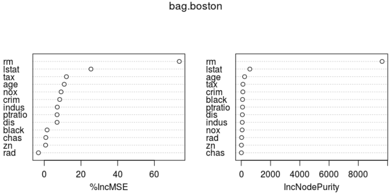
importance(bag.boston)
varImpPlot(bag.boston)
           %IncMSE IncNodePurity
crim     8.4179073    109.728304
zn       0.7225668      8.961454
indus    7.1002630     65.495428
chas     0.8471832      6.598621
nox      9.1843256     59.514880
rm      73.5567109   9626.989773
age     10.8954078    228.145275
dis      6.9800959     72.789137
rad     -3.1550071     23.389341
tax     12.0768886    115.431357
ptratio  6.9815913     84.388965
black    1.5573811     86.179297
lstat   25.4481091    586.183932
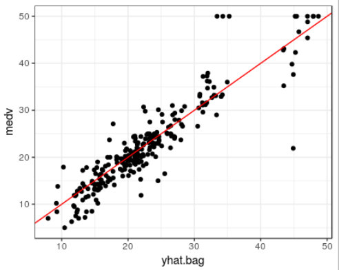
bagged model은 test데이터셋에 대한 성능은 어떠한가?
bagged regression tree에 대한 test 데이터셋의 MSE는 23.14437
(optimally-pruned single tree에서 구한 값 MSE 28.23974보다 작다.)
test
#### on Test-set
#
yhat.bag <- predict(bag.boston, newdata=boston.test)

#plot(yhat.bag, boston.test$medv); abline (0,1)
ggplot(data=boston.test, aes(x=yhat.bag, y=medv)) + theme_bw() +
    geom_point() +
    geom_abline(color="red")

mean((yhat.bag -boston.test$medv)^2)
[1] 23.14437
ntree 인수를 사용하여 randomForest()의 tree개수에 변화를 줄수 있다.
ntree : 성장한 tree의 갯수
This should not be set to too small a number, to ensure that every input row gets predicted at least a few times.
training
####################################################################
# ntree=25
### on Traing-set
nt.boston <- randomForest(medv~., data=Boston, subset =train,
                          mtry=13, importance =TRUE, ntree=25)
nt.boston
#summary(nt.boston)
#importance(nt.boston)
#varImpPlot(nt.boston)
Call:
 randomForest(formula = medv ~ ., data = Boston, mtry = 13, importance = TRUE,      ntree = 25, subset = train)
               Type of random forest: regression
                     Number of trees: 25
No. of variables tried at each split: 13

          Mean of squared residuals: 14.04305
                    % Var explained: 83
test
#### on Test-set
yhat.nt <- predict(nt.boston, newdata=boston.test)
mean((yhat.nt -boston.test$medv)^2)
[1] 13.73908
Random-Forests
Random-Forests 만들어가는 과정은 더 작은 mtry 인수값을 사용한다는 것을 제외하면, Bagging과 정확히 같다.
regression trees에 대한 Random-Forest 에서는 default로 p/3 ( 4) 이고
classification trees에 대한 Random-Forests에서는 default로 개의 변수를 사용한다.
여기서는 mtry = 6 을 적용해 봤다.
training
####################################################################
# randomForest mtry=6 importance =TRUE
#
rf.boston <- randomForest(medv~., data=Boston, subset =train,
                          mtry=6, importance=TRUE)
rf.boston
#summary(rf.boston)
Call:
 randomForest(formula = medv ~ ., data = Boston, mtry = 6, importance = TRUE,      subset = train)
               Type of random forest: regression
                     Number of trees: 500
No. of variables tried at each split: 6

          Mean of squared residuals: 11.71632
                    % Var explained: 85.81
importance(rf.boston)    # rf.boston$importance
varImpPlot(rf.boston)
          %IncMSE IncNodePurity
crim    13.689283    1228.42811
zn       2.777652      99.57551
indus   11.230307    1385.83854
chas     1.250490     124.26623
nox     13.786338    1454.47833
rm      27.377689    5525.70320
age     10.757423     630.85789
dis     14.124343    1350.70846
rad      5.422483     192.66478
tax      9.080503     657.63667
ptratio 12.567841    1248.43952
black    8.201680     427.89970
lstat   25.651663    5989.84937
importance() 함수로 변수의 중요도에 대한 2가지 측도를 살펴보면, ( varImpPlot()함수로 그래프로도 표현가능)
- %IncMSE : 주어진 변수가 model에서 제외될때 OOB(Bagging되지 않은) samples에 대한 예측 정확도의 평균 감소량에 기반
- IncNodePurity: 주어진 변수에 대한 분할로 인한 Node impurity의 총감소량을 모든 tree에 대해 평균한 값.
regression trees 의 경우, Node impurity는 Training RSS에 의해 측정
classification trees 의 경우, deviance(이탈도)에 의해 측정
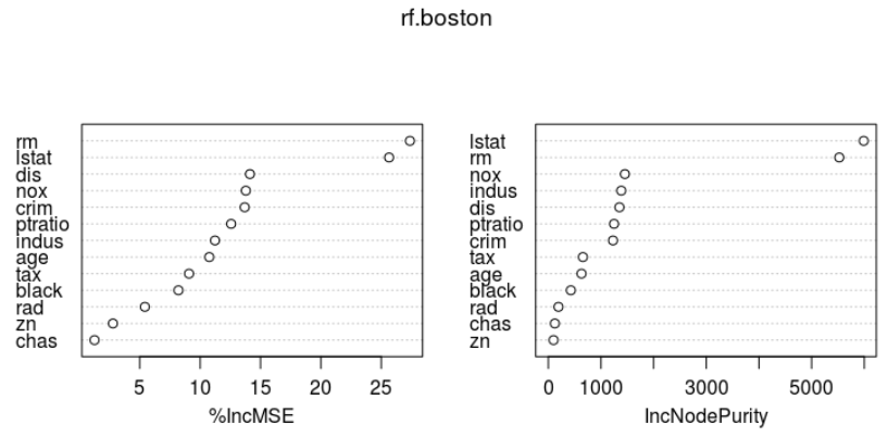
본인 소유의 주택가격(MEDV)은 하위계층의 비율(LSTAT: 재산수준)과 주택 1가구당 평균 방의 개수(RM:주택크기)가 중요한 변수이다.
test
yhat.rf <- predict(rf.boston, newdata=boston.test)
mean((yhat.rf -boston.test$medv)^2)
[1] 11.03504
test 데이터셋의 MSE는 11.03으로, Random-Forests가 Bagging보다 더 나은 결과를 보여준다.
<ALL>
####################################################################
# Boston DATA-set
library(MASS)

data("Boston")
str(Boston); head(Boston)

set.seed(1)
train <- sample(1:nrow(Boston), nrow(Boston)/2)
boston.train <- Boston[train, ]
boston.test <- Boston[-train, ]


library(ggplot2)
#install.packages("randomForest")
library (randomForest)

####################################################################
# Bagging mtry=13 importance =TRUE
#
### on Traing-set
#
bag.boston <- randomForest(medv~., data=Boston, subset =train,
                           mtry=13, importance =TRUE)
bag.boston
#summary(bag.boston)
importance(bag.boston)
varImpPlot(bag.boston)

#### on Test-set
#
yhat.bag <- predict(bag.boston, newdata=boston.test)

#plot(yhat.bag, boston.test$medv); abline (0,1)
ggplot(data=boston.test, aes(x=yhat.bag, y=medv)) + theme_bw() +
    geom_point() +
    geom_abline(color="red")

mean((yhat.bag -boston.test$medv)^2)

####################################################################
# ntree=25
### on Traing-set
nt.boston <- randomForest(medv~., data=Boston, subset =train,
                          mtry=13, importance =TRUE, ntree=25)
nt.boston
#summary(nt.boston)
#importance(nt.boston)
#varImpPlot(nt.boston)

#### on Test-set
yhat.nt <- predict(nt.boston, newdata=boston.test)
mean((yhat.nt -boston.test$medv)^2)

####################################################################
# randomForest mtry=6 importance =TRUE
#
rf.boston <- randomForest(medv~., data=Boston, subset =train,
                          mtry=6, importance=TRUE)
rf.boston
#summary(rf.boston)
importance(rf.boston)
varImpPlot(rf.boston)

yhat.rf <- predict(rf.boston, newdata=boston.test)
mean((yhat.rf -boston.test$medv)^2)
