ggplot2 default color palette

Published onesixx on 17-12-1117-12-11

# demo("colors")
# showCols1()
# grDevices::colors()
# grDevices::demo("colors")

https://stackoverflow.com/questions/25211078/what-are-the-default-plotting-colors-in-r-or-ggplot2/25211125#25211125
https://stackoverflow.com/questions/8197559/emulate-ggplot2-default-color-palette
https://stackoverflow.com/questions/33221794/separate-palettes-for-facets-in-ggplot-facet-grid

ggplot 정보 확인

p <- ggplot(iris, aes(x=Sepal.Length, y=Petal.Length, color=Species)) + geom_point()
p    
summary(p)
ggplot_build(p)$data
ggplot_build(p)$layout
ggplot_build(p)$plot

ggplot 정보 중 ggplot_build(p)$data

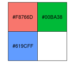
ggplot_build(p)$data

#     colour   x   y PANEL group shape size fill alpha stroke
#1   #F8766D 5.1 1.4     1     1    19  1.5   NA    NA    0.5
#...
#51  #00BA38 7.0 4.7     1     2    19  1.5   NA    NA    0.5
#...
#101 #619CFF 6.3 6.0     1     3    19  1.5   NA    NA    0.5
#...

<참고> emulate ggplot2’s default color palette

Hadley Wickham 의 ggplot1책 106 페이지

“The default colour scheme, scale_colour_hue picks evenly spaced hues around the hcl colour wheel”

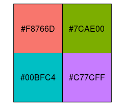
library(scales)

show_col(hue_pal()(3))
show_col(hue_pal()(4))

#[1] "#F8766D" "#00BA38" "#619CFF"
#[1] "#F8766D" "#7CAE00" "#00BFC4" "#C77CFF"

Color 설정하여 그리기

library(scales)
p <- ggplot(iris, aes(x=Sepal.Length, y=Petal.Length, color=Species))

iris2 <- cbind(iris, ggcolor=ggplot_build(p)$data[[1]][, 1])
p <- ggplot(iris2, aes(x=Sepal.Length, y=Petal.Length, color=ggcolor)) + geom_point()

color유지하면서 plot => groupOfColor

p <- ggplot(iris, aes(x=Sepal.Length, y=Petal.Length, color=Species))

groupOfColor <- ggplot_build(p)$data[[1]][, 1] %>% unique
names(groupOfColor) <- iris2$Species %>% unique
# groupOfColor

p <- ggplot(iris2, aes(x=Sepal.Length, y=Petal.Length, color=Species)) + 
    geom_point() +
    scale_color_manual(values=groupOfColor)

Manual color

data <- data.table( x=runif(10), y=runif(10), grp=factor(rep(LETTERS[1:5], each=2)))

myColors <- c("#f48025","#edd16f","#8ab96b","#4fb496","#2e74a5","#1c3d9d","#553693","#913db0",
              "#e776b9","#f78d9f","#e54d4c","#ffba57","#c2e389","#7fdfd4","#459bd8","#727ee9",
              "#b99fed","#ff99d6","#ae74e5","#8698ee","#77c7db","#559b51","#a2d252","#f0fbaf",
              "#fbdfaf","#dd5e60","#a98160","#926038" )

data %>% ggplot(aes(x=x, color=grp)) + geom_point(aes(y=y)) + 
         scale_colour_manual(values=myColors)

factor별

library(RColorBrewer)

brewer.pal.info

display.brewer.all(type="div")
display.brewer.all(type="seq")
display.brewer.all(type="qual")

display.brewer.all(10, exact.n=T)

myColors <- brewer.pal(length(levels(data$grp)), "Set1")
names(myColors) <- levels(data$grp)

myColScale <- scale_colour_manual(name="grp", values=myColors)

p1   <- data %>% ggplot(aes(x,y,color=grp)) + geom_point() + myColScale
p2_1 <- data[4:10,] %>% ggplot(aes(x,y,color=grp)) + geom_point() + myColScale
p2_2 <- p1 %+% droplevels(subset(data[4:10,]))

ggplot2 default color palette

https://stackoverflow.com/questions/25211078/what-are-the-default-plotting-colors-in-r-or-ggplot2/25211125#25211125
https://stackoverflow.com/questions/8197559/emulate-ggplot2-default-color-palette
https://stackoverflow.com/questions/33221794/separate-palettes-for-facets-in-ggplot-facet-grid

ggplot 정보 확인

ggplot 정보 중 ggplot_build(p)$data

<참고> emulate ggplot2’s default color palette

Hadley Wickham 의 ggplot1책 106 페이지

Color 설정하여 그리기

color유지하면서 plot => groupOfColor

Manual color

onesixx

ggplot2

geom_bar

ggplot2

ggplot 한글

ggplot2

Matrix with ggplot

ggplot2 default color palette

https://stackoverflow.com/questions/25211078/what-are-the-default-plotting-colors-in-r-or-ggplot2/25211125#25211125 https://stackoverflow.com/questions/8197559/emulate-ggplot2-default-color-palette https://stackoverflow.com/questions/33221794/separate-palettes-for-facets-in-ggplot-facet-grid

ggplot 정보 확인

ggplot 정보 중 ggplot_build(p)$data

<참고> emulate ggplot2’s default color palette

Hadley Wickham 의 ggplot1책 106 페이지

Color 설정하여 그리기

color유지하면서 plot => groupOfColor

Manual color

onesixx

Related Posts

ggplot2

geom_bar

ggplot2

ggplot 한글

ggplot2

Matrix with ggplot

https://stackoverflow.com/questions/25211078/what-are-the-default-plotting-colors-in-r-or-ggplot2/25211125#25211125
https://stackoverflow.com/questions/8197559/emulate-ggplot2-default-color-palette
https://stackoverflow.com/questions/33221794/separate-palettes-for-facets-in-ggplot-facet-grid