PCA 의 기본
- PCA는 차원축소에 많이 사용되지만, (PCA가 차원을 실제로 차원을 축소해 준다기 보다는)
PCA의 결과에서 차원을 선별적으로 사용한다고 이해하는 것이 좋다. - PCA는 분산이 크기로 각 차원의 데이터에 대한 설명력을 보여준다.
- PCA는 서로 직교(독립)하는 Linear 축을 찾기위해 선형변환하는 것이다.
- 즉, 각 차원의 축(PC)은 변수들의 선형결합(linear combination)이고,
X가 서로 이미 상관관계가 높지 않다면(correlation, off-diagonal 값이 0에 가까운) PCA할 이유가 없다. - (계산상으로) 직교하는 각 차원의 축(PC)는 데이터의 eigenVector이고,
설명력은 대응되는 eigenValue이다.
DATA example
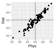
예제데이터는 학생 100명의 물리학 성적과 통계학 성적이다.
Obs의 갯수 n=100 (100명의 학생), 변수의 갯수p가 2 (ex, Phys성적, Stat성적)
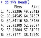
URL <- "https://raw.githubusercontent.com/steviep42/youtube/master/YOUTUBE.DIR/marks.dat"
dd <- fread(URL)
        Phys     Stat
  1: 45.83286 49.73412
  2: 66.24545 64.87357
  3: 54.84116 50.45485
  ...
 98: 29.57351 35.60014
 99: 46.26462 41.10685
100: 53.31890 48.86226
         Phys     Stat
Visualization
Original
meanPhys <- mean(dd$Phys)
meanStat <- mean(dd$Stat)

dd %>% ggplot(aes(Phys, Stat)) + geom_point() +
          geom_hline(yintercept=meanPhys, size=.3) +
          geom_vline(xintercept=meanStat, size=.3) +
          coord_equal()
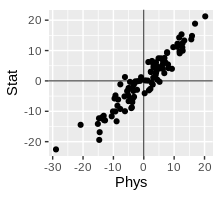
Centered (but, Not Scaled)
원래, PCA할 데이터는 표준화가 필요하다. 중심화(평균=0, center=T), 스케일 (표준편차=1, scale.=T)
이 예제에서는 일단 데이터를 중심화하고, 단위가 같기때문에 굳이 scale하진 않는다.(PCA default세팅과 같음)
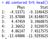
dd.centered <- dd[ ,lapply(.SD, function(x){(x-mean(x))})]
# 참고
#dd.standardize <- dd.centered.scaled <- dd[ ,lapply(.SD, function(x){(x-mean(x))/sd(x)})]

dd.centered %>% ggplot(aes(Phys, Stat)) + geom_point() +
                   geom_hline(yintercept=0, size=.3) +
                   geom_vline(xintercept=0, size=.3) +
                   coord_equal()","showLines":false,"wrapLines":false,"highlightStart":"6","highlightEnd":"7
PCA의 결과 활용
pr  <- prcomp(dd)    # center=T, scale.=F
#pr.centered <- prcomp(dd.centered)    # all.equal but pr.centerd$center

data.table(pr$x) %>%
  ggplot(aes(PC1, PC2)) + geom_point(color="blue") +
                          geom_point(data=dd.centered , aes(Phys, Stat), color="grey", alpha=0.6) +
                          coord_equal() +  geom_hline(yintercept=0, size=.3) + geom_vline(xintercept=0, size=.3)
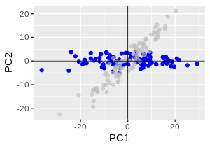
예제의 Original 데이터가 2차원이므로,
구할수 있는 PC1 PC2로 plotting하면,
선형변환을 통해 정확하게 회전만 된것으로 보여질 수 있다.
pr  <- prcomp(dd, center=F)
predict(pr)[1:6,]                         # = Score = pr$x
as.matrix(dd[1:6, ]) %*% pr$rotation      # = predict(pr)[1:6,]

predict(pr)[1:6,] %*% solve(pr$rotation)  # = dd[1:6, ]    원데이터로 원복
PCA 의미

A : 어떤 행렬
v : eigenVector
lamda : eigenValue
A : 어떤 행렬
V : eigenVectors 로 이루어진 행렬
Λ : diag() :eigenValues로 만든 대각행렬
A : 데이터의 coVariance/corRelation M, 변수들의 내적
==> cov(dd)
R : 변수의 Loading M, Rotation M, 데이터의 선형변환 , coVariance의 eigenVector
==> pr$rotation
Λ: PC의 분산으로 만든 대각행렬, 각 축의 설명력
==> diag(pr$sdev^2)
symmetric_origin <- matrix(c(-1, 0,  0, -1), nrow=2, ncol=2, byrow=T)
symmetric_xAxis  <- matrix(c( 1, 0,  0, -1), nrow=2, ncol=2, byrow=T)
symmetric_yAxis  <- matrix(c(-1, 0,  0,  1), nrow=2, ncol=2, byrow=T)
symmetric_y_x    <- matrix(c( 0, 1,  1,  0), nrow=2, ncol=2, byrow=T)

       cov(dd) %*% pr$rotation
diag(pr$sdev^2)%*% pr$rotation   # same as above

eigenV <-  eigen(cov(dd))
diag(eigenV$values) %*% eigenV$vectors %*% symmetric_origin
* Pr$x (= Scores) (=PC1 PC2... Value of the rotated data , rotated variables)
centred(또는 scaled까지)된 Original data 에 rotation matrix를 곱해서 얻은 값 (retx=TRUE일때)
pr$x                                     # the value of the rotated data
as.matrix(dd.centered) %*% pr$rotation   # same as above,
                                         # 중심화된 Data에 rotation 행렬을 곱한값, 선형변환된 결과
                                         # 실제 Phys점수 * PC1의 Phys + 실제 Stat점수 * PC1의 Stat
predict(pr)                              # same as above, Predict값
                                         #(the centred(& scaled)data multiplied by the rotation matrix)
따라서, 이미 회전을 통해 서로 Orthogonal한 축을 만들었기 때문에 cov(pr$x) 는 분산만 존재하는 diagonal matrix가 된다. 즉 diag(pr$sdev^2)
cov(pr$x)                                # cov( as.matrix(dd.centered) %*% pr$rotation )
diag(pr$sdev^2)                          # all.equal
각 PC의 설명력은 분산이고, %로 나타내면 다음과 같다.
pr$sdev^2                         #설명력, dd의 eigen-value
(pr$sdev^2)/sum(pr$sdev^2)*100
                             변수<데이터                    변수>데이터
pr$rotation             변수갯수* PC갯수(변수갯수)        변수갯수* PC갯수(데이터수)
pr$x                    데이터수* PC갯수(변수갯수)      , 데이터수* PC갯수(데이터수)
pr$sdev                     PC갯수(변수갯수)                데이터수


pr$center                    변수갯수
pr$scale                     변수갯수
| pccomp | princomp | acp | |
| rotation | loadings | loadings | the matrix of variable loadings (columns are eigenvectors) |
| eig | |||
| x | scores | scores | predict(pr) The coordinates of the individuals (obs.) on the principal components. |
| sdev | sdev | sdev | the standard deviations of the principal components |
| center | center | the variable means (means that were substracted) | |
| scale | scale | the variable standard deviations (the scaling applied to each variable ) |
참고> Data
(https://raw.githubusercontent.com/steviep42/youtube/master/YOUTUBE.DIR/BB_phys_stats_ex1.R)
그래픽으로 PCA 설명 : Explained Visually - http://setosa.io By Victor Powell with text by Lewis Lehe
txtString <- "
Phys      Stat
45.83286	49.73412
66.24545	64.87357
54.84116	50.45485
52.73309	52.98077
55.22804	57.51052
36.71771	38.1294
70.60068	71.31107
46.58481	43.0755
37.61019	37.06575
54.4459 	52.86622
42.65069	48.93422
54.37827	56.17238
55.48877	54.14389
54.75712	54.90254
58.49035	54.28524
36.50214	37.7616
57.46308	56.18982
50.88379	50.22294
66.00721	63.74446
40.21083	40.01258
62.80092	65.38431
52.6778	        53.11069
46.37766	44.08331
62.1887	        59.14436
67.25034	68.91049
46.94243	46.7534
40.7363	        44.2691
44.16992	40.07929
63.06225	61.06836
21.46127	27.51049
53.06325	56.62534
46.75746	44.27409
42.62306	40.81727
37.1718	        38.58767
35.69836	30.63126
45.89923	43.99144
58.04152	59.51573
54.64092	53.74517
41.41039	36.76394
63.12466	62.46416
41.00973	40.00774
44.99261	46.69961
44.93524	46.71632
37.29267	37.14477
58.34537	55.47421
53.43469	55.79567
45.36934	47.71729
52.06818	46.96069
49.16137	50.08758
51.86147	56.27546
56.58516	55.46879
41.69534	41.89212
62.34281	62.01932
39.80478	38.39744
56.0382	        57.49428
44.01542	44.95353
45.22847	45.33766
61.32475	61.32643
45.68322	47.66341
48.14822	47.1341
57.17597	57.60514
46.44202	41.33925
35.24607	35.90807
55.56036	49.76122
41.04521	45.28572
51.67046	50.16363
52.93516	49.51824
35.84404	33.17955
47.15922	44.82814
60.08049	61.18417
55.10556	54.57818
50.66494	46.00166
63.17677	60.00211
49.47325	51.27673
44.17665	51.33226
35.61826	37.75184
47.6078	        49.91266
62.02337	64.34087
47.17575	49.49582
59.63255	54.04946
46.66867	47.50897
41.92247	43.92537
58.06207	59.25163
63.70322	63.36367
53.54859	54.65436
54.28997	52.04134
61.45739	62.29298
48.42434	49.98111
47.02817	48.76383
56.68283	54.01947
47.39154	49.38044
53.48607	51.11642
57.12145	52.61662
62.14516	59.79395
52.54617	47.44484
56.72894	56.57045
45.37159	43.3991
29.57351	35.60014
46.26462	41.10685
53.3189	        48.86226
"
dd <- read.table(file=textConnection(txtString), header=T) %>%data.table
closeAllConnections()
library(tidyverse) library(data.table) # https://stats.stackexchange.com/questions/222/what-are-principal-component-scores txtString <- " Maths Science English Music 80 85 60 55 90 85 70 45 95 80 40 50 " dd <- read.table(file=textConnection(txtString), header=T) %>% as.data.table() closeAllConnections() dd pr <- prcomp(dd, scale. = T) pr$x pr$rotation pr$sdev cov(dd) %*% pr$rotation symmetric_origin <- matrix(c(-1, 0, 0, -1), nrow=2, ncol=2, byrow=T) symmetric_xAxis <- matrix(c( 1, 0, 0, -1), nrow=2, ncol=2, byrow=T) symmetric_yAxis <- matrix(c(-1, 0, 0, 1), nrow=2, ncol=2, byrow=T) symmetric_y_x <- matrix(c( 0, 1, 1, 0), nrow=2, ncol=2, byrow=T)
