data.table join(merge)
Inner join: merge(x = df1, y = df2, by = "CustomerId")
merge(x = df1, y = df2, by.x="keyx", by.y="keyy")
Cross join: merge(x = df1, y = df2, by = NULL)
Outer join: merge(x = df1, y = df2, by = "CustomerId", all = TRUE)
Left outer: merge(x = df1, y = df2, by = "CustomerId", all.x = TRUE)
Right outer: merge(x = df1, y = df2, by = "CustomerId", all.y = TRUE)
suffixes=c("x",".y")
data.table의 merge()는 기본모듈인 merge() 과 유사하지만,
data.frame에 기반한 basic merge()는 data.frame내에 변수를 pk로 사용하여 merge하는데 비해
data.table의 Merging은 common key variable 을 pk로 사용하여 merge한다는 점이 다르다.
Key확인 – tables()
setkey는 data.table의 Key로써 A, B를 지정한다. (이 id 변수로 그룹화의 기준으로 생각하면 된다.)
all set* functions change their input by reference
Fast add/ remove/ update subsets of columns, by reference. :=
> key(dt1)
> key(dt2)
[1] "A"

> tables()              # KEY column reports the key'd columns
     NAME NROW NCOL MB COLS KEY
[1,] dt1     6    2  1 A,X  A
[2,] dt2     6    2  1 A,Y  A
Total: 2MB
update using Two tables
dt1 <- data.table( A=letters[rep(1:3,2)], X=1:6, key="A")
dt2 <- data.table( A=letters[rep(2:4,2)], Y=6:1, key="A")

dt1 <- data.table( A=letters[rep(1:3,2)], X=1:6) ; setKey(dt1, "A")   # same as above
dt2 <- data.table( A=letters[rep(2:4,2)], Y=6:1) ; setKey(dt2, "A")
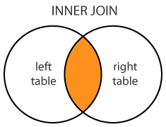
Inner Join
merge(dt1, dt2, by="A")
merge(dt1, dt2)             # setKey된 A로 merge
dt1[dt2, on=.(A), nomatch=0] # no match row is not returned
   A X Y
1: b 2 6
2: b 2 3
3: b 5 6
4: b 5 3
5: c 3 5
6: c 3 2
7: c 6 5
8: c 6 2
(Left) OUTER JOIN
merge(dt1, dt2, by="A", all.x = T)
dt2[dt1, on="A"]
   A X  Y        A  Y X
 1: a 1 NA     1: a NA 1
 2: a 4 NA     2: a NA 4
 3: b 2  6     3: b  6 2
 4: b 2  3     4: b  3 2
 5: b 5  6     5: b  6 5
 6: b 5  3     6: b  3 5
 7: c 3  5     7: c  5 3
 8: c 3  2     8: c  2 3
 9: c 6  5     9: c  5 6
10: c 6  2    10: c  2 6
Right (OUTER) JOIN
merge(dt1, dt2, by="A", all.y = T)
dt1[dt2, on="A"]
    A  X Y
 1: b  2 6
 2: b  2 3
 3: b  5 6
 4: b  5 3
 5: c  3 5
 6: c  3 2
 7: c  6 5
 8: c  6 2
 9: d NA 4
10: d NA 1
Full (OUTER) JOIN
merge(dt1, dt2, all=T)
    A  X  Y
 1: a  1 NA
 2: a  4 NA
 3: b  2  6
 4: b  2  3
 5: b  5  6
 6: b  5  3
 7: c  3  5
 8: c  3  2
 9: c  6  5
10: c  6  2
11: d NA  4
12: d NA  1
https://github.com/Rdatatable/data.table/wiki/Getting-started
https://stackoverflow.com/questions/1299871/how-to-join-merge-data-frames-inner-outer-left-right
https://stackoverflow.com/questions/8508482/what-does-sd-stand-for-in-data-table-in-r
https://www.analyticsvidhya.com/blog/2016/05/data-table-data-frame-work-large-data-sets/
Use of lapply .SD in data.table R
HTML vignettes: https://github.com/Rdatatable/data.table/wiki/Getting-started
>
>
>
>
>
>
Creates a Join data table
J {data.table}
DT = data.table(x=rep(c("b","a","c"),each=3),
                y=c(1,3,6),
                v=1:9)
#row selection like join
DT[x=="a"]
DT["a",    on="x"]
DT[.("a"), on="x"]
DT[J("a"), on="x"]

setkey(DT, "x")
tables()
DT["a"]
DT[.("a")]
DT[J("a")]
   x y v
1: a 1 4
2: a 3 5
3: a 6 6
4: b 1 1
5: b 3 2
6: b 6 3
7: c 1 7
8: c 3 8
9: c 6 9
x y v
1: a 1 4
2: a 3 5
3: a 6 6J : (J)oin.
the same result as calling list. J is a direct alias for list but results in clearer more readable code.
SJ : (S)orted (J)oin.
The same value as J() but additionally setkey() is called on all the columns in the order they were passed in to SJ.
For efficiency, to invoke a binary merge rather than a repeated binary full search for each row of i.
CJ : (C)ross (J)oin.
A data.table is formed from the cross product of the vectors.
For example, 10 ids, and 100 dates, CJ returns a 1000 row table containing all the dates for all the ids.
It gains sorted,
which by default is TRUE for backwards compatibility. FALSE retains input order.
DT = data.table(x=rep(c("b","a","c"),each=3),
                y=c(1,3,6),
                v=1:9)
#row selection like join
DT[x=="a"]
DT["a",    on="x"]
DT[.("a"), on="x"]
DT[J("a"), on="x"]

setkey(DT, "x")
tables()
DT["a"]
DT[.("a")]
DT[J("a")]
Join 시 Match되지 않는 데이터 처리
- 기본적으로 NA로 return된다.
- NA로 처리될 row를 지워버릴수 있다.
- roll을 통해 다른 값을 대체할수 있다.
(LOCF) last observation carried forward => +Inf (or TRUE) 마지막값으로
(NOCB)next observation carried backward => -Inf
rolls the nearest value instead. => "nearest"
DT[.("b", 1:2), on=c("x", "y")]             # no match returns NA
   x y  v
1: b 1  1
2: b 2 NA

DT[.("b", 1:2), on=.(x, y), nomatch=0]      # no match row is not returned
x y v
1: b 1 1

DT[.("b", 1:2), on=c("x", "y"), roll=Inf]   # locf, nomatch row gets rolled by previous row
x y v
1: b 1 1
2: b 2 1

DT[.("b", 1:2), on=.(x, y), roll=-Inf]      # nocb, nomatch row gets rolled by next row
x y v
1: b 1 1
2: b 2 2
Inner join: df1[df2, on=.("CustomerId"), nomatch=0L]
Outer join: merge(x = df1, y = df2, by = "CustomerId", all = TRUE)
Left outer: merge(x = df1, y = df2, by = "CustomerId", all.x = TRUE)
Right outer: dt1[dt2, on=.("CustomerId")]
Cross join: merge(x = df1, y = df2, by = NULL)
dtProd <-  data.table(CustomerId = c(1:6),   Product= c(rep("iphone",3), rep("gallaxy",3)) )
dtAddr <-  data.table(CustomerId = c(3,5,7), Address= c(rep("Seoul",2),  rep("Pusan", 1))  )

# full outer join
merge(dtProd, dtAddr, by="CustomerId", all=T)
merge(dtProd, dtAddr, by=c("CustomerId", "Sex"), all=T)

# inner join
merge(dtProd, dtAddr, by="CustomerId")
dtProd[dtAddr, nomatch=0L, on="CustomerId"]

# anti join - use `!` operator
dtProd[!dtAddr, on="CustomerId"]

### outer join
# right outer join (unkeyed)
dtProd %>% setkey(NULL)
dtAddr %>% setkey( NULL)
dtProd[dtAddr, on = "CustomerId"]

# right outer join (keyed data.tables)
dtProd %>% setkey(CustomerId)
dtAddr %>% setkey(CustomerId)
dtProd[dtAddr]

# left outer join - swap dt1 with dt2
dtAddr[dtProd, on = "CustomerId"]
join(merge)
dtProd <-  data.table(CustomerId = c(1:6),   Product= c(rep("iphone",3), rep("gallaxy",3)) )
dtAddr <-  data.table(CustomerId = c(3,5,7), Address= c(rep("Seoul",2),  rep("Pusan", 1))  )

# full outer join
merge(dtProd, dtAddr, by="CustomerId", all=T)
merge(dtProd, dtAddr, by=c("CustomerId", "Sex"), all=T)

# inner join
merge(dtProd, dtAddr, by="CustomerId")
dtProd[dtAddr, nomatch=0L, on="CustomerId"]

# anti join - use `!` operator
dtProd[!dtAddr, on="CustomerId"]


### outer join
# right outer join (unkeyed)
dtProd %>% setkey(NULL)
dtAddr %>% setkey( NULL)
dtProd[dtAddr, on = "CustomerId"]

# right outer join (keyed data.tables)
dtProd %>% setkey(CustomerId)
dtAddr %>% setkey(CustomerId)
dtProd[dtAddr]

# left outer join - swap dt1 with dt2
dtAddr[dtProd, on = "CustomerId"]
data.table의 Merging은 기본모듈인 merge() 과 유사하지만,
dataframe에 기반한 basic merge()는 data.frame내에 변수를 pk로 사용하여 merge하는데 비해
data.table의 Merging은 common key variable 을 pk로 사용하여 merge한다는 점이 다르다.
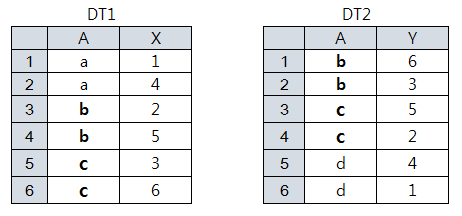
Example Data
dt1 <- data.table( A=letters[rep(1:3,2)], X=1:6, key="A")
dt2 <- data.table( A=letters[rep(2:4,2)], Y=6:1, key="A")

dt1 <- data.table( A=letters[rep(1:3,2)], X=1:6)
setKey(dt1, "A")
dt2 <- data.table( A=letters[rep(2:4,2)], Y=6:1)
setKey(dt2, "A")
dt1 A X        dt2 A Y
 1: a 1         1: b 6
 2: a 4         2: b 3
 3: b 2         3: c 5
 4: b 5         4: c 2
 5: c 3         5: d 4
 6: c 6         6: d 1
all set* functions change their input by reference.
Fast add, remove and update subsets of columns, by reference. :=
Key확인
key(dt1)
key(dt2)
[1] "A"
tables() # KEY column reports the key'd columns
     NAME NROW NCOL MB COLS KEY
[1,] dt1     6    2  1 A,X  A
[2,] dt2     6    2  1 A,Y  A
Total: 2MB
update using Two tables
Inner Join
merge(dt1, dt2, by="A")
merge(dt1, dt2)             # setKey된 A로 merge
   A X Y
1: b 2 6
2: b 2 3
3: b 5 6
4: b 5 3
5: c 3 5
6: c 3 2
7: c 6 5
8: c 6 2
Outer join: merge(x = df1, y = df2, by = "CustomerId", all = TRUE)
Left outer: merge(x = df1, y = df2, by = "CustomerId", all.x = TRUE)
Right outer: merge(x = df1, y = df2, by = "CustomerId", all.y = TRUE)
Cross join: merge(x = df1, y = df2, by = NULL)
Subscript Method
A left outer join with df1 on the left using a subscript method would be:
df1[,"State"]<-df2[df1[ ,"Product"], "State"]The other combination of outer joins can be created by mungling the left outer join subscript example. (yeah, I know that's the equivalent of saying "I'll leave it as an exercise for the reader...")
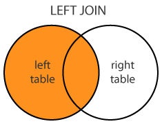
Left (OUTER) JOIN
merge(dt1, dt2, by="A", all.x = T)

    A X  Y
 1: a 1 NA
 2: a 4 NA
 3: b 2  6
 4: b 2  3
 5: b 5  6
 6: b 5  3
 7: c 3  5
 8: c 3  2
 9: c 6  5
10: c 6  2
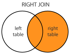
Right (OUTER) JOIN
merge(dt1, dt2, by="A", all.y = T)

dtResult <- dt1[dt2,        on="A"]             # [.data.table
dtResult <- dt1[dt2,      , on="A"]
dtResult <- dt1[dt2,.(X,Y), on="A"]
dtResult <- dt1[dt2, .(X, i.Y), on="A"]         # i.Y = dt2.Y
    A  X Y
 1: b  2 6
 2: b  2 3
 3: b  5 6
 4: b  5 3
 5: c  3 5
 6: c  3 2
 7: c  6 5
 8: c  6 2
 9: d NA 4
10: d NA 1
Full (OUTER) JOIN
merge(dt1, dt2, all=T)
    A  X  Y
 1: a  1 NA
 2: a  4 NA
 3: b  2  6
 4: b  2  3
 5: b  5  6
 6: b  5  3
 7: c  3  5
 8: c  3  2
 9: c  6  5
10: c  6  2
11: d NA  4
12: d NA  1
예제 Data : 야구 데이터 (from Lahman)
특정 column만 뽑아내기는 data.frame과 data.table이 조금 다르다.
library(Lahman)
data("Pitching")

# Extract specific column
setDF(Pitching)
P0 <-  Pitching[ , c('playerID', 'yearID', 'teamID', 'W', 'L', 'G', 'ERA')]

setDT(Pitching)
P1 <-  Pitching[ , .(playerID, yearID, teamID, W, L, G, ERA)]
예제 Data : data.table
library(data.table)
set.seed(666)
DT <- data.table( A=rep(c("a","b","c"),each=2), B=c(1:3), C=sample(6), D=sample(6))
setkey(DT, A, B)
setkey는 data.table의 Key로써 A, B를 지정한다. 은 id 변수로 그룹화의 기준으로 생각하면 된다.
Roll
Join 시 Match되지 않는 데이터 처리
- 기본적으로 NA로 return된다.
- NA로 처리될 row를 지워버릴수 있다.
- Roll을 통해 다른 값을 대체할수 있다.
(LOCF) last observation carried forward => +Inf (or TRUE) 마지막값으로
(NOCB)next observation carried backward => -Inf
rolls the nearest value instead. => "nearest"
DT[.("b", 1:2), on=c("x", "y")]             # no match returns NA
   x y  v
1: b 1  1
2: b 2 NA

DT[.("b", 1:2), on=.(x, y), nomatch=0]      # no match row is not returned
x y v
1: b 1 1

DT[.("b", 1:2), on=c("x", "y"), roll=Inf]   # locf, nomatch row gets rolled by previous row
x y v
1: b 1 1
2: b 2 1

DT[.("b", 1:2), on=.(x, y), roll=-Inf]      # nocb, nomatch row gets rolled by next row
x y v
1: b 1 1
2: b 2 2
. (dot)
가끔 regression formulas에서 볼수 있었던 (ex. lm(y~., data=DT) ) . 는"all other variables"을 의미하지만,
data.table에서는 "list"를 의미한다. any*는 .( ) 를 활용
DT[ , .(x, y)]
DT[ , list(x, y)]       # identical
.SD (Subset of Data)
.SD는 하나의 data.table의 columns을 각각 sub data.table로 나누어 self reference할수 있게 해준다.
subsetting
: .SD만 단순히 사용하면, 원래 값과 같다.
DT
DT[ , .SD]             # identical
   A B C D
1: a 1 1 3
2: a 2 6 6
3: b 3 5 4
4: b 1 3 2
5: c 2 4 1
6: c 3 2 5
self reference
: A column와 B column을 paste하는 것을 .SD를 활용하여 같은 결과를 구현할수 있다.
paste(DT$A,DT$B,sep="")
DT[ , .SD[ , paste(A,B,sep="")], ]      # identical
[1] "a1" "a2" "b3" "b1" "c2" "c3
.SDcols
column subsetting
DT[ , .SD, .SDcols=c("B","C","D")]
DT[ , .SD[ ,c("B","C","D")] ]            # identical
   B C D
1: 1 2 1
2: 2 5 3
3: 3 1 6
4: 1 4 5
5: 2 6 4
6: 3 3 2
ex> Sum all columns
DT[ , lapply(.SD, sum)]        # data.table
DT[ , colSums(.SD)]            # vector
 B  C  D
12 21 21
lapply 활용
.SD는 lapply에서 Column 기준으로 반복
DT[, lapply(.SD, function(x){is.numeric(x)})]
       A    B    C    D
1: FALSE TRUE TRUE TRUE
Sum A columns
DT[ , lapply(.SD, sum), .SDcols=2]
DT[ , lapply(.SD, sum), .SDcols="B"]
    B
1: 12
Sum all columns EXCEPT A
DT[ , lapply(.SD, sum), .SDcols=!"A"]
    B  C  D
1: 12 21 21
grouping BY A => Sum all columns EXCEPT A
DT[ , lapply(.SD, sum), by=A]
   A B  C D
1: b 4 10 5
2: a 3  6 9
3: c 5  5 7
Sum all columns EXCEPT A, grouping BY B
DT[ , lapply(.SD, sum), by=B, .SDcols=!"A"]
   B  C  D
1: 1 11 10
2: 2  4  5
3: 3  6  6
:= data의 불필요한 Copy를 방지
data.table's reference semantics vignette
Subsetting의 인덱싱 결과는 또 다른 새로운 data.table이다.(즉 원래 DT에 재할당하지 않는 이상, DT는 변하지 않고 유지된다)
따라서, DT의 size가 big한 경우, := 를 사용하여 컬럼을 참조하여 update함으로써 data의 불필요한 Copy를 방지한다.
DT[ , names(DT):= lapply(.SD, as.factor) ]
row selection
sub-data.table의 row index를 활용하여 dynamically하게 원하는 row만 뽑아올수 있다.
아래는 각 그룹의 B열에서 max값을 갖는 row를 뽑아오는 예제.
DT[, .SD[which.max(B)], by=A]
   A B C D
1: a 2 4 5
2: b 3 3 3
3: c 3 5 1
DT[, .(max(B)), by=A]
DT[, lapply(.SD, max), .SDcols=c('B'), by=A]
DT[, lapply(.SD, function(x){B=max(x)}), .SDcols=c('B'), by=A]
   A B
1: a 2
2: b 3
3: c 3
Convert Column Type
여러 방법을 통해 out_idx를 정의하고, 해당 컬럼에 함수(as.factor)를 적용하여, column type을 covert한다.
data.table이 각 element가 column인 list로 여겨질수 있다는 것이다.
(out_idx)를 괄호로 감싸는 이유는 컬럼명으로 인식하게 하기 위해.
#1. 컬럼 직접 지정
out_idx <- c('A')
out_idx <- c(1)
#2. type확인하여 컬럼 지정
out_idx <- which(sapply(DT, is.character))
#3.  colname의 패턴으로 컬럼 지정
out_idx <- grep('A', names(DT))
out_idx <- grep('A', names(DT), value=T)    # value=F는 index값

DT[ , (out_idx):=lapply(.SD, as.factor), .SDcols=out_idx]
Data.Frame을 사용해서도 같은 결과를 얻을수 있다.
setDF(DT)                              # convert to data.frame for illustration
sapply(DT[ ,out_idx], is.character)
SD[.N]
.N 은 그룹내의 전체row갯수 . 즉 그룹별로 nrow(.SD)한것과 같다.
ex)
.SD[.N] 은 각 그룹내의 마지막 row값(관측값, obs)을 나타내고, .SD[1L] 은 각 그룹내에 첫번째 관측값을 나타낸다.
DT %>% nrow    # 6

DT[ , .SD[.N], ]
DT[ , .SD[6],  ]
DT[ 6, ]

DT[, .SD[.N], by=A]
DT[c(2,4,6), ]
Performance check
# 10*6 data.table
DT <- replicate(6, sample(seq(100L),10,T)) %>% as.data.table
DT[ , LETTERS[1:2] := .(sample(100L,10,T), sample(100L,10,T))]

# 10000000 * 6  더 큰 데이터테이블 만들기
kk = seq(100L)
nn = 1e7
DT <- replicate(6, sample(kk,nn,T)) %>% as.data.table
DT[ , LETTERS[1:2]:=.(sample(kk,nn,T), sample(kk,nn,T))]

library(microbenchmark)
microbenchmark(times = 100L,
               colsums  = colSums(DT[ , !c("A", "B"), with = FALSE]),
               colsums2 = DT[ , colSums(.SD), .SDcols=!c("A", "B")],
               lapplys  = DT[ , lapply(.SD, sum), .SDcols = !c("A", "B")])
Unit: milliseconds
     expr       min        lq      mean    median        uq       max neval cld
  colsums 215.75608 216.39019 222.84491 216.99909 221.86177 395.47297   100   c
 colsums2 164.90262 165.44731 166.86141 165.72122 166.05506 181.50616   100  b
  lapplys  36.02945  36.82467  37.44593  37.20621  37.45793  48.53117   100 a
